###The definition of B-Spline curve
$$\vec{C}(u)=\sum _{i=0}^n N_{i,p}(u) \vec{P}_i \text{ }\qquad (0\leq u\leq 1)$$
where, $\vec{P}_i$ is the control point, and the $N_ {i, p} (u)$ are the $p$-th - degree B-spline basis functions defined on the non-periodic(and non-uniform) knot vector $U$.
$$U=\{\underbrace {0,\cdots ,0}_{p+1},u_{p+1},\cdots u_{m-p-1},\underbrace {1,\cdots,1}_{p+1}\}$$
For the non-rational B-spline curve of degree $p$, its derivative is a $p-1$ degree non-rational curve. where, the new control points and knot vector are $Q_i$ and $U'$, respectively. $$\vec Q_i=p \frac{\vec P_{i+1}-\vec P_i}{u_{i+p+1}-u_{i+1}}$$
$$U'=\{\underbrace {0,\cdots ,0}_{p},u_{p+1},\cdots u_{m-p-1},\underbrace {1,\cdots,1}_{p}\}$$
I think the built-in f = BSplineFunction[2D/3D-points vector]; f' just returns a non-rational curve.
However, for the rational B-spline curve: $$\vec{C}^w(u)=\frac{\sum_{i=0}^n N_{i,p}(u)w_i\vec{P}_i}{\sum_{i=0}^n N_{i,p}(u)w_i}=\frac{\vec{A}(u)}{w(u)}$$
where, $\vec P_i=\{x_i, y_i\}$(2D curve) or $\vec P_i=\{x_i, y_i,z_i\}$(3D curve). Then
$$\left[\vec{C}^w(u)\right]'=\left[\frac{\vec A(u)}{w(u)}\right]'=\frac{\vec A'(u)w(u)-\vec A(u)w'(u)}{w^2(u)}$$
The derivative of built-in BSplineFunction[] for curve case is right when the weights is vector that contains same value. Namely, the curve is non-rational.
Here, ptsW = wi {xi, yi, zi}
BSplineDer[pts_, wgts_, {deg_, knots_}][u_?NumericQ] :=
 Module[{ptsW, A, w, Au, wu, AuDer, wuDer},
  ptsW = pts wgts;
  A = BSplineFunction[ptsW, SplineDegree -> deg, SplineKnots -> knots];
  w = BSplineFunction[wgts, SplineDegree -> deg, SplineKnots -> knots];
 (*calculate the A(u) and w(u)*)
  Au = A[u];
  wu = w[u];
  (*calculate the derivative of A(u) and w(u)*)
  AuDer = A'[u];
  wuDer = w'[u];
  (*using the NURBS curve derivative formula*)
  (wu AuDer - wuDer Au)/wu^2
]
###TEST
pts = {{1, 1}, {2, 3}, {3, -1}, {4, 1}, {5, 0}};
wgts = {1, 2, 3, 4, 5};
knots = {0, 0, 0, 0, 0.5, 1, 1, 1, 1};
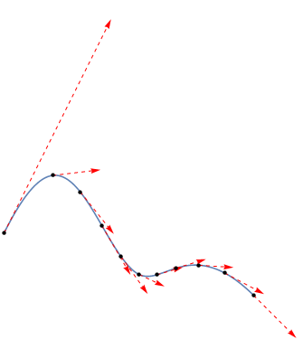
f = BSplineFunction[pts, SplineDegree -> 3, SplineWeights -> {1, 2, 3, 4, 5}]

Show[
 {ParametricPlot[f[t], {t, 0, 1}],
  Graphics[
   {Red, Dashed, Arrowheads[0.03],
    Table[Arrow[{f[t], f[t] + BSplineDer[pts, wgts, {3, knots}][t]/7}], {t, 0, 1, 0.1}]}],
  ListPlot[f /@ Range[0, 1, 0.1],
   PlotStyle -> Directive[Black, PointSize[Medium]]]},
 PlotRange -> All, Axes -> False
]

