## Another update ##
Not sure when this was introduced, but copying the demo figure provided above from your browser window to Mathematica using copy and paste results in each pixel being defined by 4 values instead of usual three RGB values. I suppose the fourth is an alpha channel used for opacity. This is not the case if you `Import` using the image link.
Getting the image using copy and paste also provides the image with options that differ by version. In 11.3 the options are `{ColorSpace -> "RGB", Interleaving -> True}`, whereas in 13.3.1 the options are `{ColorSpace -> "RGB", ImageResolution -> {96., 96.}, ImageSize -> {353.438, Automatic}, Interleaving -> True}`. This causes problems with the `ImageTrim` function and everything following that. It explains the issue Kvothe reported in the comments below.
The workaround is either importing the image using its link or getting rid of the alpha layer and the `ImageResolution` option using something like:
im2 = Image[ImageData[im][[All, All, ;; 3]],
{ColorSpace -> "RGB", Interleaving -> True}
]
where `im` is assigned to the copy-and-pasted figure.
For me, this makes it work again.
## UPDATE: Added a few workarounds for bugs / features introduced in Mathematica v10 or later.
##
Main issue involved `LocatorPane` whose `Appearance` option no longer correctly handles more than one `Graphics` object [CASE:4984027]. This bug was introduced somewhere after v11.3 and is present in v.13.1. Additional issues concerned the scaling of the graphics used in the various panels, which was incorrect. Perhaps a different default was introduced somewhere after v9 where the code worked as intended.
----------
----------
**Original text**
Here the contours of a method to do this half-automatic selection you are looking for. It is heavily based on an example on the `ImageCorrelate` doc page of Waldo fame. First, you interactively select an example of the plot marker you want to look for:
img = Import["https://i.sstatic.net/hhPr9.png"];
pt = {ImageDimensions[img]/4, ImageDimensions[img]/2};
LocatorPane[
Dynamic[pt],
Dynamic[
Show[
img,
Graphics[
{
EdgeForm[Black], FaceForm[], Rectangle @@ pt
}
]
]
], Appearance -> Graphics[{Red, AbsolutePointSize[5], Point[{0, 0}]}]
]
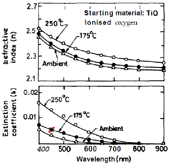
Then you use Mathematica v8's image processing tools to find similar structures:
res =
ComponentMeasurements[
MorphologicalComponents[
ColorNegate[
Binarize[
ImageCorrelate[
img,
ImageTrim[img, pt],
NormalizedSquaredEuclideanDistance
], 0.18
]
]
], {"Centroid", "Area"}, #2 > 1 & (*use only the larger hits*)
];
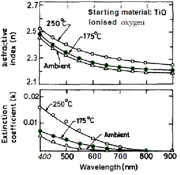
The coordinates are now in `res`. I'll show them below. Many are correct, sometimes you get some spurious hits and misses. It depends on the `Binarize` threshold value and the "Area" size chosen in `ComponentMeasurements` third argument.
Show[img, Graphics[{Green, Circle[#, 5] & /@ res[[All, 2, 1]]}]]
----
**EDIT:** Here a more complete application. It is not robust as it is (no error handling at all), but nevertheless already quite useful.
The function `getMarkers` is called with an image as argument and the name of a variable in which the final markers are returned:

You get the app with tabs that represent processing stages:
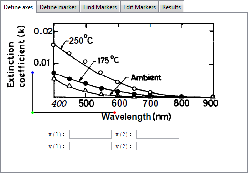
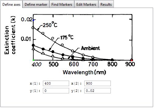
In the first tab you define the axes by dragging the colored dots to the locations on the x and y axis with the highest known value and to the origin of the plot. Here, you also enter the values for the bottom left and top right corners of the rectangle that they define:
In the next tab you then indicate the marker you want to have detected:
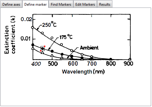
The detection results are presented in the next tab and you can drag a slider to increase or decrease the number of results:
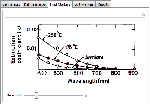
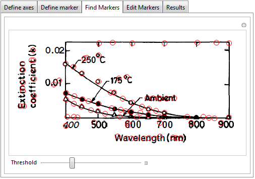
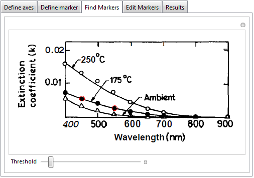
You can manually adjust the detected markers in the next tab. Markers can be dragged, removed (alt-click an existing marker) and added (alt-click on an empty spot). Actually, this is so easy to do that I would be tempted to say that I could do without the marker-detection phase.
The end result can be seen in the Results tab. If something is wrong you can go back to an earlier tab:
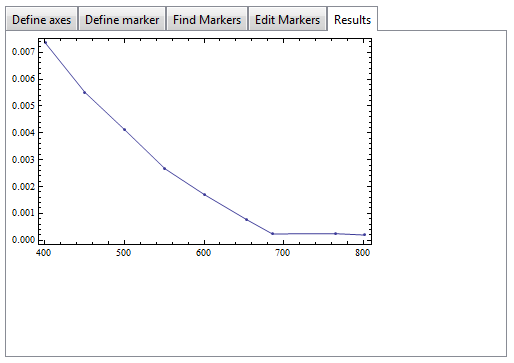.
The data plotted in the Results tab is also copied in the variable passed to the function, test in this example.
test
(*
==> {{400.5159959, 0.007353847123}, {450.3095975,
0.005511544915}, {499.8452012, 0.004129136525}, {550.9287926,
0.002664992936}, {600.4643963, 0.001702431875}, {653.869969,
0.000764540446}, {685.6037152, 0.0002398789942}, {764.7123323,
0.0002481309886}, {801.7027864, 0.0001989932135}}
*)
The code:
findMarkers[img_, pt_, thres_, minArea_] :=
ComponentMeasurements[
MorphologicalComponents[
ColorNegate[
Binarize[
ImageCorrelate[img, ImageTrim[img, pt],
NormalizedSquaredEuclideanDistance
], thres]
]
],
{"Centroid", "Area"},
#2 > minArea &
][[All, 2, 1]];
SetAttributes[getMarkers, HoldRest];
getMarkers[img_, resMarkers_] :=
DynamicModule[
{
pt = {ImageDimensions[img]/4, ImageDimensions[img]/2},
axisDefinePane, defineMarkerPane, findMarkerPane, editMarkersPane,
finalResultPane, xAxisBegin, xAxisEnd, yAxisBegin, yAxisEnd,
myMarkers, myTransform,
xoy = {{1/2, 1/8} ImageDimensions[img], {1/8, 1/8} ImageDimensions[
img], {1/8, 1/2} ImageDimensions[img]}},
axisDefinePane =
Grid[
{
{
LocatorPane[
Dynamic[xoy],
Dynamic[
Show[
img,
Graphics[{Line[xoy]}],
ImageSize -> ImageDimensions[img]
]
],
Appearance ->
{
Graphics[{AbsolutePointSize[5], Red, Point[{0, 0}]}],
Graphics[{AbsolutePointSize[5], Green, Point[{0, 0}]}],
Graphics[{AbsolutePointSize[5], Blue, Point[{0, 0}]}]
}
]
},
{Row[{"x(1): ",
InputField[Dynamic[xAxisBegin], Number, FieldSize -> Tiny],
" x(2): ",
InputField[Dynamic[xAxisEnd], Number,
FieldSize -> Tiny]}]}, {Row[{"y(1): ",
InputField[Dynamic[yAxisBegin], Number, FieldSize -> Tiny],
" y(2): ",
InputField[Dynamic[yAxisEnd], Number,
FieldSize -> Tiny]}]}}];
defineMarkerPane =
LocatorPane[
Dynamic[pt],
Dynamic[
Show[
img,
Graphics[{EdgeForm[Black], FaceForm[], Rectangle @@ pt}],
ImageSize -> ImageDimensions[img]
]
],
Appearance -> Style["\[FilledSmallCircle]", Red]
];
findMarkerPane =
Manipulate[
Show[
img,
Graphics[{Red,
Circle[#, 5] & /@ (myMarkers = findMarkers[img, pt, t, 1.05])}],
ImageSize -> ImageDimensions[img]
],
{{t, 0.2, "Threshold"}, 0, 1},
TrackedSymbols -> {t},
ControlPlacement -> Bottom
];
editMarkersPane =
LocatorPane[
Dynamic[myMarkers],
img,
Appearance ->
Graphics[{Red, Circle[{0, 0}, 1]}, ImageSize -> 10],
LocatorAutoCreate -> True
];
finalResultPane =
Dynamic[
myTransform =
FindGeometricTransform[{{xAxisEnd, yAxisBegin}, {xAxisBegin,
yAxisBegin}, {xAxisBegin, yAxisEnd}}, xoy][[2]] // Quiet;
ListLinePlot[resMarkers = myTransform /@ Sort[myMarkers],
Frame -> True, Mesh -> All, ImageSize -> ImageDimensions[img]],
TrackedSymbols -> {myMarkers, xoy, xAxisEnd, yAxisBegin,
xAxisBegin, yAxisBegin, xAxisBegin, yAxisEnd}
];
TabView[
{
"Define axes" -> axisDefinePane,
"Define marker" -> defineMarkerPane,
"Find Markers" -> findMarkerPane,
"Edit Markers" -> editMarkersPane,
"Results" -> finalResultPane
}
]
]