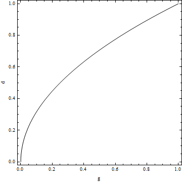
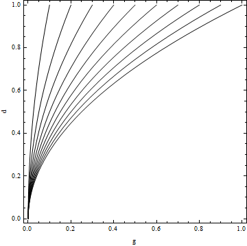
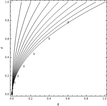
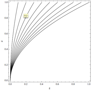
I'm revisiting this topic because I have a new solution at the bottom of the post. The outline of this answer is:
Interactively labeling contours
- Using the graphics editor
- Using
Tooltip
- Converting
Tooltip displays to static labels at custom positions
Section 1 was my original answer, the other two are new.
1. Using the graphics editor
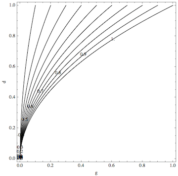
What I usually do is label the contours by hand with the help of the drawing tools. For that you first have to know what labels belong to which contour. In your example, the label you want is the parameter t, so to get myself oriented I first defined a ContourLabels function that can display that number:
labelFunction[t_][x_, y_, z_] := Text[t, {x, y}]

Show[Table[
  ContourPlot[t*d^2 - g, {g, 0, 1}, {d, 0, 1}, Contours -> {0},
   ContourStyle -> Black, ContourShading -> None,
   FrameLabel -> {"g", "d"}, ContourLabels -> labelFunction[t]], {t,
   0.1, 1, 0.1}]]

I left all the other things unchanged in your example.
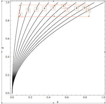
Then I re-did the plot without ContourLabels (just delete that option), and highlighted the resulting plot by clicking on it. Next, press t and click where you want to add the first manually placed contour label. Type the number for the contour, and click outside the text to accept the label. press t again to start adding the next contour label at your desired position, etc.

After entering the labels like this, you can also double-click each label and edit it further, e.g. by moving it around if you don't like your original choice of placement.
How permanent are these annotations?
One problem that always makes me feel uneasy about using the editing tools is that manual annotations appear less permanent because they don't get reproduced when you re-run the notebook. However, it's worth pointing out that manual annotations aren't all that bad in practice:
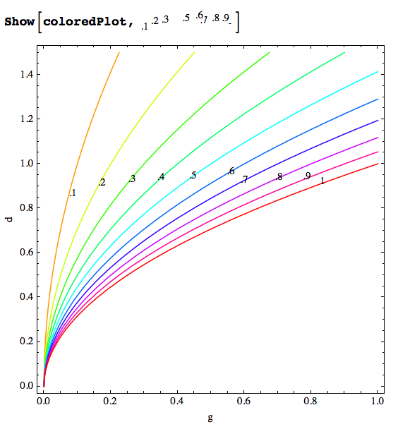
Assume you want to re-do the last plot above, keeping the labels but coloring the contours differently. The colors could be added like this:
coloredPlot =
 Show[Table[
   ContourPlot[t*d^2 - g, {g, 0, 1}, {d, 0, 1.5}, Contours -> {0},
    ContourStyle -> Hue[t], ContourShading -> None,
    FrameLabel -> {"g", "d"}], {t, 0.1, 1, 0.1}]]
Note that I added ContourStyle -> Hue[t] and also changed the plot range in the vertical direction. But now of course the labels are gone again. Fortunately, you can copy the contour labels from the previous plot as follows:

Here I double clicked one label, then shift-clicked the others to select them all. Now I pressed the copy keyboard shortcut and go back to the colored plot coloredPlot I just produced.
Next, type the following:

Here, I pasted the previously copied labels into the Show command. Executing this line, I get the labels at the correct absolute plot coordinates in the new plot.
The conclusion from this is that the manual labor involved in making the labels as I showed above is not completely wasted when you re-draw the contour plot, because copying your work preserves the coordinates of the insets.
2. Using Tooltip
Normally, Tooltip is the easiest way to label contours because that's the default behavior of ContourPlot when no ContourLabels option is specified.
However, we want to label contours by a Tooltip showing a custom quantity, not the default which is contour height. In the documentation for ContourLabels (under Details), you find that custom tool tips should be available by specifying
ContourLabels -> {f, g}
where the second function, g, is used "as a tooltip for each complete contour line." This is very ambiguously worded, and it seems to have had people stumped (see the MathGroup archive). It turns out that g isn't the function that specifies the argument for the Tooltip, it actually has to be of Head Tooltip.
So in the example of the question, for a Table of several contour plots where each contour is custom labeled by the Table index t, we can get a tooltip-labeled plot like this:
toolPlot = Show[
 Table[
  ContourPlot[t*d^2 - g, {g, 0, 1}, {d, 0, 1}, Contours -> {0},
   ContourStyle -> Black, ContourShading -> None,
   FrameLabel -> {"g", "d"},
   ContourLabels -> {
     None,
     Tooltip[#, t] &}
   ],
  {t, 0.1, 1, 0.1}
  ]
 ]

The first function in ContourLabels is simply set to None so we don't get any static labels at all. The second argument shows how you get the Tooltip labeling "each complete contour line," as the documentation put it.
Now we're done debugging the mysterious documentation, and it's time for the fun part:
3. Converting Tooltip displays to static labels at custom positions
Here we ask the question:
Given a graphics object such as toolPlot from above, can we convert the information contained in the Tooltips into static labels and position these labels interactively?
This is different from adding labels completely manually, because we're going to rely on the auto-generated information in the Tooltip and only leave the choice of position as a manual task.
For this, I'll use the same idea as in my answer to this question, but modified to get a dynamically updated graphic that includes labels wherever I click on a Tooltip-decorated line:
Options[burnTooltips] = {ImageSize -> 360,
   "LabelFunction" -> (Framed[#, FrameStyle -> None,
       RoundingRadius -> 8, Background -> RGBColor[1, .8, .4]] &)};

burnTooltips[plot_, opt : OptionsPattern[]] := DynamicModule[
  {
   ins = {},
   wrapper = OptionValue["LabelFunction"],
   toolRule = Function[{arg},
     Tooltip[t__] :> Button[
       Tooltip[t],
       AppendTo[
        arg,
        Inset[wrapper[Last[{t}]], MousePosition["Graphics"]]
        ]
       ],
     HoldAll]
   },
  EventHandler[
   Dynamic@Show[
     plot /. toolRule[ins],
     Graphics@ins,
     ImageSize -> OptionValue[ImageSize]
     ],
   {"MouseUp", 2} :> (toolRule = {} &)
   ]
  ]
The function burnTooltips can be applied to the contour plots of our example as follows:
burnTooltips[toolPlot]
This will display the graphic in the argument again, but now whenever you click on an object displaying a Tooltip, the displayed value appears as a static label in the graphic. When you're done adding the labels at locations where they look good to you, you may want to prevent this dynamic display from receiving any further clicks. To do that, right-click the mouse over the completed picture.
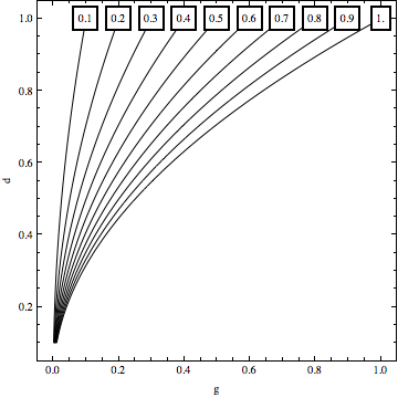
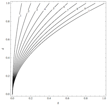
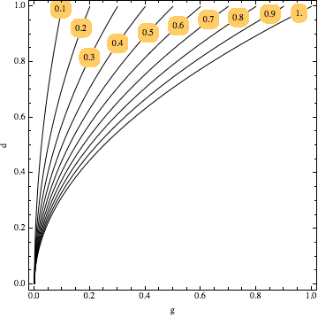
Here is what the result might look like:

To continue working with this graphic, copy it and paste it into the next Input cell. For example, to get an image to upload above, I typed
Export["picture.png", ]
and pasted the image in the space.
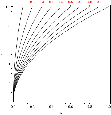
There are two options you may want to play with for burnTooltips: ImageSize and "LabelFunction". The first one doesn't need explanation, and the second one should be something of the type Framed[#]& or Pane[#]& (my default setting is shown in the image). By adding the label formatting as a function (note the &), it's possible to customize the labels almost arbitrarily. For example, one could also try this:
"LabelFunction" -> (Pane[Style[#, Red, Background -> White],
    ImageSize -> {20, 20}, ImageSizeAction -> "ResizeToFit"] &)
This method is pretty amenable to how I normally work with plots: use default labeling (i.e., Tooltip in this case) while exploring the problem, and start worrying about the exact placement of labels only at the end.
Here I showed how one can get to the finalized labeled plot from the Tooltip stage. In the function burnTooltips, the Tooltip is used as a kind of vehicle with which a new "payload" can be injected into an existing plot, turning it into a dynamic object that accumulates information about where you click to place labels containing the exact same information that the Tooltip displayed.
Generalizations
You should be able to apply burnTooltips to virtually any Graphics object, not just ContourPlots. But I think ContourPlot is one of the most important applications for this technique because even in single plots (not tables as we considered here), the automatically generated labels are often placed in awkward locations so that manual adjustment is required.
