20
$\begingroup$

The problem is from Principles of Statistics by M.G. Bulmer:

In a certain survey of the work of chemical research workers, it was found, on the basis of extensive data, that on average each man required no fume cupboard for 60 per cent of his time, one cupboard for 30 per cent and two cupboards for 10 per cent; three or more were never required. If a group of four chemists worked independently of one another, how many fume cupboards should be available in order to provide adequate facilities for at least 95 per cent of the time?

My approach to solving it has been to enumerate, for the 4 chemists, all the cases in which each requires 0, 1 or 2 fume cupboards. This takes the form of a list like so:

{{0,0,0,0}, {0,0,0,1}, {0,0,0,2}, {0,0,1,0}, {0,0,1,1}, {0,0,2,0},...}

I then compute the probability of each particular case, sort the cases from low to high by number of cupboards required, and finally compute a running cumulative probability:

(* enumerate all the cases, as length-4, base-3 numbers *)
hoods = PadLeft[IntegerDigits[#, 3], 4, 0] & /@ Range[0, 80];

(* compute overall odds per case *)
odds = {0 -> 0.6, 1 -> 0.3, 2 -> 0.1};
data = Table[{
    Plus @@ x, x, x /. odds, Times @@ (x /. odds)}, 
    {x, hoods}];

(* sort by number of hoods needed for each case *)
data = Sort[data, #1[[1]] < #2[[1]] &];

(* compute & thread in cumulative probability the N hoods will be enough *)
cumulativeOdds = Accumulate[#[[4]] & /@ data];
data = Flatten[#, 1] & /@ Thread@{Range[1, 81], cumulativeOdds, data};

headings = {"idx", "cum. prob.", "hoods needed", 
   "hoods per chemist", "prob./chemist", "overall prob."};

Grid[Prepend[data, headings], Frame -> All, 
    Background -> {None, {51 -> LightRed}}, Spacings -> {1.5, 1.2}]

table top

table middle

My question is: is there a more direct way to approach this kind problem, perhaps using higher-level Mathematica features/functions or higher-level concepts from probability?

Followup:

I made a table and graph summarizing Eric Towers' Excellently Simple & Short Solution:

pdf = CoefficientList[(0.6 + 0.3 x + 0.1 x^2)^4, x];
cdf = Accumulate[pdf]; len = Length[pdf];
tbl = Table[{i - 1, pdf[[i]], cdf[[i]]}, {i, 1, len}];
Grid[{{tbl // TableForm, ListPlot[Transpose@tbl[[All, {2, 3}]],
    AxesOrigin -> {-1, 0}, DataRange -> {0, len - 1}, 
    ImageSize -> 250]}}, Spacings -> 4]
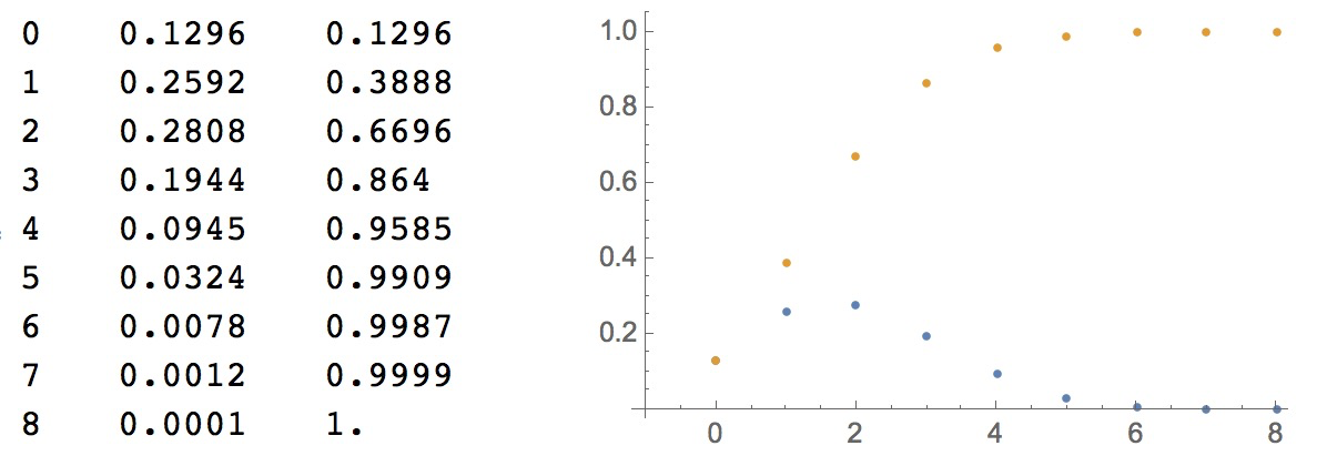
table and plot

$\endgroup$

4 Answers 4

26
$\begingroup$
dist = TransformedDistribution[b + 2 c, {a, b, c} \[Distributed] 
                               MultinomialDistribution[4, {.6, .3, .1}]];

Reduce[CDF[dist, x] >= .95, x]

(* x>=4 *)

Check:

CDF[dist, 4]
(* .9585 *)

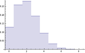
The PMF:

DiscretePlot[PDF[dist, x], {x, 0, 8}, ExtentSize -> All, PlotRange -> All]

enter image description here

Explanation:

MultinomialDistribution[4, {.6, .3, .1}]

Defines the base distribution - we're taking 4 samples (the four participants) from a distribution with each having a .6/.3/.1 probability of getting catagory 1/2/3 (corresponding to none, 1, and 2 hoods needed).

TransformedDistribution[b + 2 c, {a, b, c} \[Distributed] 
                                   MultinomialDistribution[4, {.6, .3, .1}]];

takes this into an algebra on the random variable (we'll get some number of category 1 (a) worth zero, some number of category 2 (b) worth 1, and some number of category 3 (c) worth 2) - so 0*a+1*b+2*c hoods total for some realization of the variable. The 0*a is obviously 0, so the sum we're after is simply b+2c. The TransformedDistribution gives us that sum, itself a random variable.

Reduce[CDF[dist, x] >= .95, x]

solves for where in the distribution the Cumulative Distribution Function (the probability for all realizations of x at or below something) is >=.95, our desired threshold. N.b.: This appears to be one of those cases where the more typical Quantile or InverseCDF returns unevaluated - MMA does not handle this particular transform for those, so Reduce fills those shoes.

And, in the spirit of "... higher-level concepts from probability..." (though I'd venture it's a stretch to call this such), a direct appeal to the multinomial expansion:

Table[{n, N@Tr@Select[CoefficientRules[(.3 o + .1 t + .6 z)^4], 
                  Total[#[[1]]*{1, 2, 0}] <= n &][[All, 2]]}, {n, 0, 8}]

(*
{{0,0.1296},{1,0.3888},{2,0.6696},{3,0.864},
 {4,0.9585},{5,0.9909},{6,0.9987},{7,0.9999},{8,1.}}
*)

Or, by convolution of the PMF:

Accumulate@Nest[ListConvolve[#, {.6, .3, .1}, {1, -1}, 0] &, {.6, .3, .1}, 3]

(* {0.1296,0.3888,0.6696,0.864,0.9585,0.9909,0.9987,0.9999,1.} *)

The same (convolution), but appealing to the Fourier Transform, so we need not nest explicitly (and depending on the problem, can have great performance benefits):

ps = {.6, .3, .1};
num = 4;
asize = 2^Ceiling[Log2[num]*(Length@ps - 1)];
padded = PadRight[ps, asize];
fourier = Sqrt[asize] Fourier[padded];
Accumulate@TakeWhile[Chop@InverseFourier[fourier^num]/Sqrt[asize], # != 0 &]

(* {0.1296,0.3888,0.6696,0.864,0.9585,0.9909,0.9987,0.9999,1.} *)

I suppose a "higher level concept" might be complex probabilities, so for complete LOLs, here's the result using them combined with the Poisson-Binomial Distribution (I won't clutter with code, pbpmf2 is just the referenced distribution, with an additional argument of the weights (4 each))

pbpmf2[{a, b} /. Solve[a + b - 2 a b == 3/10 && a*b == 1/10, {a, b}] //
         First, {4, 4}] // Accumulate // N // Chop

(* {0.1296,0.3888,0.6696,0.864,0.9585,0.9909,0.9987,0.9999,1.} *)

Another way would be using a Markov Chain:

mc = PadRight[
   Join[PadLeft[{.6, .3, .1}, #] & /@ 
     Range[3, 9], {{0, 0, 0, 0, 0, 0, 0, 1}, {0, 0, 0, 0, 0, 0, 0, 0,1}}]];

dmc = DiscreteMarkovProcess[1, mc];

Table[{n - 1, CDF[dmc[4], n]}, {n, 1, Length@mc}]

(* {{0,0.1296},{1,0.3888},{2,0.6696},{3,0.864},{4,0.9585},{5,0.9909},{6,0.9987},{7,0.9999},{8,1}} *)

Finally, in the spirit of "... higher-level Mathematica features/functions...", the result via our own distribution definition:

dz = ProbabilityDistribution[
   Piecewise[{{.6, x == 0}, {.3, x == 1}, {.1, x == 2}}], {x, 0, 2, 1}];

dx = ProductDistribution[{dz, 4}];

Table[{n, Probability[user1 + user2 + user3 + user4 <= n, 
                     {user1, user2, user3, user4} \[Distributed] dx]}, {n, 0, 8}]

(*
{{0,0.1296},{1,0.3888},{2,0.6696},{3,0.864},
 {4,0.9585},{5,0.9909},{6,0.9987},{7,0.9999},{8,1.}}
*)
$\endgroup$
24
  • 4
    $\begingroup$ @J.M. Oh. Heh. I should Destroy All Evidence but I'll leave it for other people's amusement instead. :^) $\endgroup$
    – Mr.Wizard
    Commented Jul 14, 2015 at 8:26
  • 1
    $\begingroup$ Ah, Quantile[]/InverseCDF[] doesn't work… damn, that's another bug on my gedanken version… :D $\endgroup$ Commented Jul 14, 2015 at 8:26
  • 1
    $\begingroup$ @J.M. Agreed - neat question, fun burning a cigar and a half pondering differing ways... $\endgroup$
    – ciao
    Commented Jul 14, 2015 at 10:17
  • 1
    $\begingroup$ @billc, allow me to assure you that the next time somebody asks me "how do I ask a good question?", I will be citing this as one example. $\endgroup$ Commented Jul 16, 2015 at 5:16
  • 1
    $\begingroup$ ... Although this leads to a complex solution like {1/20 (5 - I Sqrt[15]), 1/20 (5 + I Sqrt[15])}, this can still be used in the Poisson Binomial calculation. Using my implementation: PoissonBinomialPDF[{1/20 (5 - I Sqrt[15]), 1/20 (5 + I Sqrt[15])}] ==>{0.6, 0.3, 0.1}, and for 4 chemists: PoissonBinomialCDF[ Table[{1/20 (5 - I Sqrt[15]), 1/20 (5 + I Sqrt[15])}, {4}] // Flatten] ==>{0.1296, 0.3888, 0.6696, 0.864, 0.9585, 0.9909, 0.9987, 0.9999, 1.} $\endgroup$ Commented Nov 20, 2016 at 15:55
13
$\begingroup$

I think this is one way to approach the problem but I am by no means an expert in this area.

dd =
 MixtureDistribution[{60, 30, 10}, DiscreteUniformDistribution[{#, #}] & /@ {0, 1, 2}];

N @ Probability[w + x + y + z <= n, # \[Distributed] dd & /@ {w, x, y, z}]

$\begin{array}{cc} \{ & \begin{array}{cc} 0.1296 & 0.\leq n<1. \\ 0.3888 & 1.\leq n<2. \\ 0.6696 & 2.\leq n<3. \\ 0.864 & 3.\leq n<4. \\ 0.9585 & 4.\leq n<5. \\ 0.9909 & 5.\leq n<6. \\ 0.9987 & 6.\leq n<7. \\ 0.9999 & 7.\leq n<8. \\ 1. & n\geq 8. \\ 0. & \text{True} \\ \end{array} \\ \end{array}$

$\endgroup$
1
  • $\begingroup$ thanks @Mr.Wizard ... much for me to learn from here. $\endgroup$
    – billc
    Commented Jul 14, 2015 at 17:53
9
$\begingroup$

We can encode one chemist's need of fume cupboards with $0.6 + 0.3 c + 0.1 c^2$. Since they work independently, we may find their simultaneous needs via multiplication:

ExpandAll[(0.6 + 0.3 c + 0.1 c^2)^4]
(* Output:  0.1296 + 0.2592 c + 0.2808 c^2 + 0.1944 c^3 + 0.0945 c^4 + 
            0.0324 c^5 + 0.0078 c^6 + 0.0012 c^7 + 0.0001 c^8 *)

from which we see several things we know. No hoods are needed $0.6^4 \approx 0.1296$ of the time. No more than eight fume cupboards are ever needed (and then only $0.1^4 = 0.0001$ of the time). Accumulating coefficients from the constants end, we cross 0.95 at $c^4$ and likewise accumulating from the highest degree end we cross 0.05 at $c^4$. Thus, four cupboards satisfy demand at least 95% of the time. We can make the computer show us this via

Accumulate[CoefficientList[ExpandAll[(0.6 + 0.3 c + 0.1 c^2)^4],c]]
(* Output:  {0.1296, 0.3888, 0.6696, 0.864, 0.9585, 0.9909, 0.9987, 0.9999, 1.} *)

Note that this method can be used for mixtures of chemists with different requirements. So, three chemists requiring 0 or 2 cupboards each half the time and two chemists with the 60%/30%/10% profile of the problem give

Accumulate[CoefficientList[ExpandAll[(0.6 + 0.3 c + 0.1 c^2)^2 (0.5 + 0.5 c^2)^3],c]]
(* Output:  {0.045, 0.09, 0.25125, 0.39375, 0.60875, 0.76625, 0.89375, 0.96125, 0.99125, 0.99875, 1.} *)

aren't 95% satisfied with fewer than 7 fume cupboards.

We can also mix in additional constrained resources. Suppose in the original problem that a chemist using one fume cupboard requires six big beakers ($b$) and one using two fume hoods requires four big beakers. From the encoding $0.6+0.3c b^6 + 0.1 c^2 b^4$, we get

Accumulate[CoefficientList[Expand[(0.6 + 0.3 c b^6 + 0.1 c^2 b^4)^4], c]]
(* Output:  Hard to interpret mess.  *)

Suppose we decide to have an abundance of beakers. Then we set $b \rightarrow 1$ and get the above result. Suppose we can only afford 20 big beakers. Then $b^{n\_}/;n>20 \rightarrow 0, b^{n\_}/;n<=20 \rightarrow 1$ gives us

Accumulate[CoefficientList[Expand[(0.6 + 0.3 c b^6 + 0.1 c^2 b^4)^4], c]/.
    {b^n_ /; n > 20 -> 0, b^n_ /; n <= 20 -> 1}
]
(* Output:  {0.1296, 0.3888, 0.6696, 0.864, 0.9504, 0.972, 0.9798, 0.981, 0.9811}  *)

and 4 hoods (barely) meets our 95% criterion. Repeating with 16 big beakers, we can never reach 95% utilization no matter how many hoods we have. To find the frontier, we can make a table...

TableForm[
    Accumulate[
        Accumulate /@ 
            CoefficientList[Expand[(0.6 + 0.3 c b^6 + 0.1 c^2 b^4)^4], {c, b}]
    ],
    TableHeadings -> {Range[0, 8], Range[0, 24]}
]
(* Output:  Happy to let someone else put this here; I'm not up to that much typing. *)

and we discover 95% utilization is hopeless with fewer than 18 big beakers (by running our finger along the last row) or fewer than 4 fume cupboards (by running our finger along the last column). This is not the generic behaviour. The generic behaviour gives a tradeoff (more hoods and fewer beakers or vice versa) between resources. I'm too lazy to adjust this example to show this behaviour.

Edit: For further reading, see Generating Functions and Probability-generating Functions

$\endgroup$
3
  • $\begingroup$ A lovely, clear method. Note that you do not need Expand or ExpandAll when using CoefficientList however so this can be made cleaner still. $\endgroup$
    – Mr.Wizard
    Commented Jul 15, 2015 at 0:17
  • $\begingroup$ Nicely done, +1 $\endgroup$
    – ciao
    Commented Jul 15, 2015 at 0:49
  • $\begingroup$ Thanks! This is very cool. I converted your first two examples to a small table: clst = CoefficientList[ExpandAll[(0.6 + 0.3 x + 0.1 x^2)^4], x]; Thread@{Range[0, 8], clst, Accumulate[clst]} // TableForm $\endgroup$
    – billc
    Commented Jul 15, 2015 at 6:30
6
$\begingroup$

Just a simulation...not as nice as any of the given answers (which I have upvoted...I liked @ciao (rashers) MultinomialDistribution transformed {0,1,2}.{a,b,c}.

p[n_, s_] := 
 With[{t = 
    Total /@ RandomChoice[{0.6, 0.3, 0.1} -> {0, 1, 2}, {s, 4}]}, 
  N@Total@Boole[Thread[t <= n]]/s]

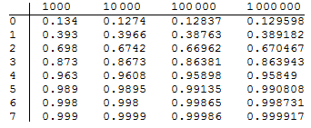
Calculation of probabilities of success with n fume cabinets:

With[{r = PowerRange[1000, 1000000]}, 
 TableForm[Table[p[j, #] & /@ r, {j, 0, 7}], 
  TableHeadings -> {Range[0, 7], r}]]

enter image description here

$\endgroup$
1
  • $\begingroup$ Ah - I'd completely neglected simulations, +1 $\endgroup$
    – ciao
    Commented Jul 14, 2015 at 22:44

Your Answer

By clicking “Post Your Answer”, you agree to our terms of service and acknowledge you have read our privacy policy.

Not the answer you're looking for? Browse other questions tagged or ask your own question.