25
$\begingroup$

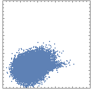
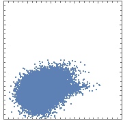
Consider the following scatterplot of a 50K-point dataset:

ListPlot[data,
 AspectRatio -> Automatic, PlotRange -> {{x0, x1}, {y0, y1}}, 
 ImageSize -> Small,
 Frame -> True, 
 FrameTicksStyle -> Directive[FontOpacity -> 0, FontSize -> 0]]
Mathematica graphics

The color quickly saturates as one moves from the edge of the distribution to its center. As a result, most of the density information is lost.

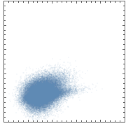
One can remedy this slightly by assigning an opacity below 1 to the points:

ListPlot[data,
 PlotStyle -> Opacity[0.05],
 AspectRatio -> Automatic, 
 PlotRange -> {{x0, x1}, {y0, y1}}, ImageSize -> Small,
 Frame -> True, 
 FrameTicksStyle -> Directive[FontOpacity -> 0, FontSize -> 0]]

Mathematica graphics

But this solution still has a couple of shortcomings:

  1. its dynamic range is still fairly narrow (even though it's wider than it was before); thus, most of the data cloud is still shows as saturated color;
  2. there's no explicit quantitative scale (e.g. a colorbar) tying colors (or in this case, shades) to densities;

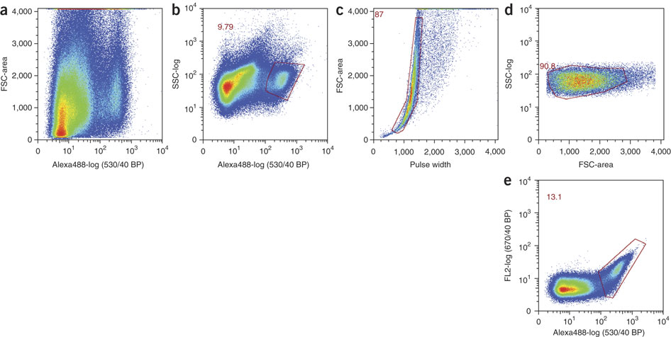
The dynamic range problem could be solved by using more hues. This is what's routinely done when plotting flow cytometry data. For example:
enter image description here

(IMO, the plots in the last set would be improved if they included a color key, showing the correspondence between colors and densities.)

My question is how can I provide such quantitative density information in these scatterplots using Mathematica?

$\endgroup$
2

4 Answers 4

25
$\begingroup$

I think SmoothDensityHistogram (docs here) is what you are looking for:

data1 = RandomVariate[BinormalDistribution[{0, 0}, {2, 3}, 0.5], 100000];
data2 = RandomVariate[BinormalDistribution[{3, 4}, {2, 2}, .1], 100000];
data = data1~Join~data2;

This is just some random sample data. If you plot it using ListPlot, you obtain the "blob" you mentioned:

ListPlot[data, AspectRatio -> 1]

Mathematica graphics

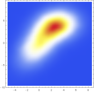
Here is the same data presented with a smoothed 2D-histogram instead:

SmoothDensityHistogram[data, ColorFunction -> "TemperatureMap"]

Mathematica graphics


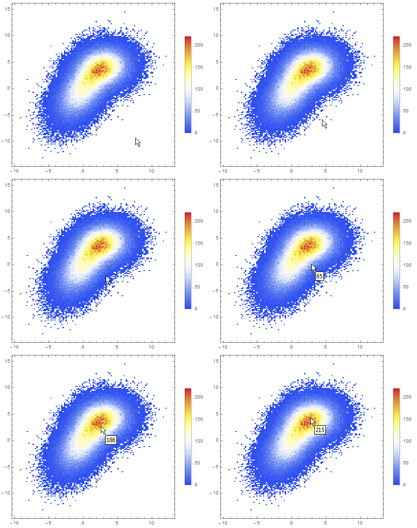
Data comparison: Jim Baldwin brought up a good point in comments regarding the need to compare multiple datasets, both visually and numerically. In that case, DensityHistogram may be the best bet. This function essentially is the discrete version of SmoothedDensityHistogram; the advantage in this context is the fact that it also has built-in tooltips whose value can be configured to report on distribution properties such as the total counts in each bin, probability, the value of the probability density function calculated from the data distributions, etc. In particular, this function may be most interesting because it can automatically generate legends for its data as shown below. Here is the documentation for DensityHistogram.

For instance, using the data above:

DensityHistogram[data, "Wand", "Count", 
    ColorFunction -> "TemperatureMap", 
    ChartLegends -> Automatic
]

density histogram with tooltip and legend

Instead of "Count", one could also request the bin height to represent the PDF, CDF, etc. In this case I chose Wand binning among the built-in options because to me it seemed to offer the best compromise between fine-grained binning that reproduced the overall "shape" of the data, and execution time (ca. 7s on my machine). Knuth binning looked even better, but it took almost one minute to calculate on the same dataset!

In passing, I'd also like to mention that these *DensityHistogram functions seem to work very similarly under the hood, differing mostly in the way they present the data. In particular, my understanding is that both start by recovering a smooth kernel distribution from the existing data, using a Gaussian kernel by default.

Alternatively, other approaches focused on layering contour lines on top of a smooth density histogram have also been discussed in this question (Contour lines over SmoothDensityHistogram) to which Jim and others have contributed interesting answers.

$\endgroup$
3
  • $\begingroup$ This will give a good visual feel for the density but if a more quantitative approach is desired, then I'd repeat my above comment that SmoothKernelDistribution would allow for drawing contours that enclosed a specified proportion of points or a specified volume (probability). This becomes more important if two or more datasets are being compared and need comparable coloring/contour schemes. (But maybe there's an option for a SmoothDensityHistogram that allows one to specify contour heights.) $\endgroup$
    – JimB
    Commented Jun 9, 2015 at 15:34
  • $\begingroup$ @JimBaldwin I think you make an excellent point regarding the comparisons. I believe that this can be addressed from within the *DensityHistogram functions themselves (please take a look at the updated version of my answer). What do you think? $\endgroup$
    – MarcoB
    Commented Jun 9, 2015 at 16:54
  • $\begingroup$ Very good update. And by "numerically" (rather than "visually") I was referring to things like "the smallest area under the surface that encompasses 95% of the probability" which are used in animal home ranges as opposed to the height of the probability surface. So rather than contours at fixed and uniformly spaced heights/elevations, a set of contours with associated coverage probabilities is sometimes more desirable. (And as been pointed out by others, desirable things also depend on the objectives rather than just the data.) $\endgroup$
    – JimB
    Commented Jun 9, 2015 at 17:16
12
$\begingroup$

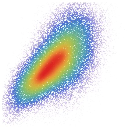
It looks like kjo did something very similar.

data1 = RandomVariate[BinormalDistribution[{0, 0}, {2, 3}, 0.5], 100000];
data2 = RandomVariate[BinormalDistribution[{3, 4}, {2, 2}, 0.1], 100000];
data = data1~Join~data2;

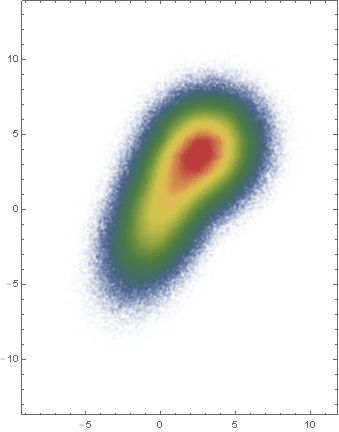
Module[{vals, vc, f},
 f = PDF[SmoothKernelDistribution[data, PerformanceGoal -> "Speed"]];
 vals = Rescale[ParallelMap[f, data]];
 vc = ParallelMap[Directive[Opacity[#], ColorData["DarkRainbow"][#]] &, vals];
 Graphics[Point[data, VertexColors -> vc], Frame -> True]
 ]

enter image description here

$\endgroup$
1
  • $\begingroup$ +1 ! The combination of opacity and color is a surprising twist. $\endgroup$
    – kjo
    Commented Jun 9, 2015 at 17:40
11
$\begingroup$

OK, I figured out a solution, based on Jim Baldwin's suggestion (and borrowing a trick from Lebesgue ;-) ).

The basic idea is this:

  1. use SmoothKernelDistribution to get a density function for the data;
  2. use this function to classify the original data points into level sets according to their probability density;
  3. the final plot is a composite of the plots of the various level sets, each getting an appropriate color.

In the implementation below, I've factored out the generation of the level sets into a separate function.

densityLevelSets[data_, nlevelsets_] :=
  Module[
    { 
      distribution = SmoothKernelDistribution[data, PerformanceGoal -> "Speed"]
    , n = Length[data]
    , d
    , dmin
    , drange
    , z
    , zmax = nlevelsets - 1
    }
    , d = PDF[distribution, #] & /@ data
    ; dmin = Min[d]
    ; drange = Max[d] - dmin
    ; z = Min[Floor[nlevelsets ((# - dmin)/drange)], zmax]& /@ d
    ; data[[#]] & /@ (Values @ KeySort[GroupBy[Range[n], z[[#]]&]])
];

Now, with this function in hand, we can plot something like this:

With[{nlevelsets = 20},
  ListPlot[densityLevelSets[data, nlevelsets],
   PlotStyle -> Table[ColorData["StarryNightColors"][i/nlevelsets],
                      {i, nlevelsets}],
   AspectRatio -> Automatic,
   PlotRange -> {{x0, x1}, {y0, y1}},
   Frame -> True,
   FrameTicksStyle -> Directive[FontOpacity -> 0, FontSize -> 0]
  ]
]

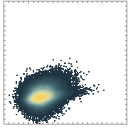
Mathematica graphics

Here's the comparison with the plotting methods described in the original post:

Mathematica graphics Mathematica graphics Mathematica graphics


This is only a partial solution, because the density levels are now computed relative to a single dataset. IOW, there is no global density scale that would allow a fair comparison of densities between two different plots.

But the elements of the full solution are all there, I think.

EDIT: Nicked the PerformanceGoal->"Speed" optimization from chuy's answer. EDIT: Fixed bug in densityLevelSets function; simplified it substantially.

$\endgroup$
3
  • 1
    $\begingroup$ kjo, that's a neat approach, but it seems to me that you could let Mathematica do more of the heavy lifting for you ;-) $\endgroup$
    – MarcoB
    Commented Jun 9, 2015 at 17:11
  • 2
    $\begingroup$ Not sure why you say "there is no global density scale that would allow a fair comparison between two different plots." A nonparametric density estimate (SmoothKernelDistribution) scales everything so that the volume under the surface is 1.0. This means one can compare heights of the surfaces and areas that contain a specified probability among any number of datasets. $\endgroup$
    – JimB
    Commented Jun 9, 2015 at 17:23
  • $\begingroup$ @JimBaldwin: in general, you're right; I was referring specifically to my implementation above, which renormalizes the density to maximize the dynamic range for an individual plot. $\endgroup$
    – kjo
    Commented Jun 9, 2015 at 17:27
5
$\begingroup$

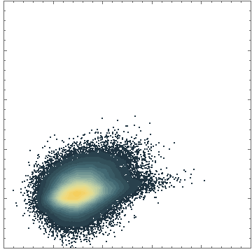
In the interest of providing yet-another-method™, here's the crazy Image/Colour processing approach that first popped into my head after reading @chuy's answer (mainly because Opacity directives are pretty slow on my machine). Not so much a complete answer to the problem, as I haven't worked out frames and other luxuries, but an alternative route that somebody might want to explore at some point:

prange = {{-5, 10}, {-5, 10}};
toimg[plt_] := Image[plt, ImageSize -> 512];
 {img1, img2, mask} = toimg /@
  {SmoothDensityHistogram[data, PlotRange -> prange, Frame -> None, ColorFunction -> "Rainbow"],
   Graphics[Point[data], PlotRange -> prange],
   SmoothDensityHistogram[data, PlotRange -> prange, Frame -> None, ColorFunction -> "GrayTones"]};

SetAlphaChannel[ColorReplace[ImageMultiply[ImageAdd[img1, img2],
 Binarize@ColorNegate@img2], Black -> White],
 ImageMultiply[ImageAdjust@mask, 5.5]]

enter image description here

$\endgroup$

Your Answer

By clicking “Post Your Answer”, you agree to our terms of service and acknowledge you have read our privacy policy.

Not the answer you're looking for? Browse other questions tagged or ask your own question.