Generating evenly spaced points on a curve

Question

In the KnotData package a simple command such as

points = Table[KnotData[{3, 1}, "SpaceCurve"][t], {t, 0, 2 Pi, 0.1}];

will generate a series of points that comprise a knot (here, a trefoil, if successive points are connected).

However, the distance between points is not constant; is there a way to generate evenly spaced points? (I.e. evenly spaced arc lengths between points).

Answer 1

I'm going to brute force it numerically.

First, let's define the function we're interested in:

fun = KnotData[{3, 1}, "SpaceCurve"]

Imagine that this function fun[t] describes the position of a moving point in time. The the magnitude of its velocity as a function of the time t is

Sqrt[#.#] & [fun'[t]]

I'm going to make an interpolating function out of this to speed up and simplify the numerical calculations:

v = FunctionInterpolation[Sqrt[#.#] & [fun'[t]], {t, 0, 2 Pi}]

The integral (antiderivative) of this function will give us the distance covered as a function of time.

dist = Derivative[-1][v]

This is a monotonically increasing function, so it can be inverted:

invdist = InverseFunction[dist]

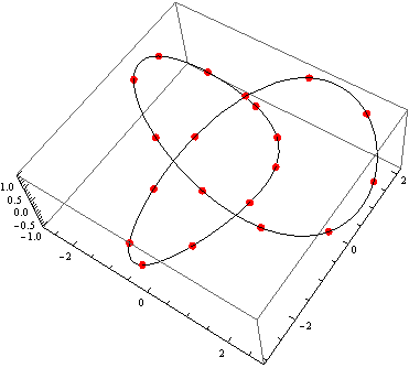
Using the inverse we can generate the times at which the point passes through the equally spaced points. Let's divide the curve into 20 equal-length segments:

times = Table[invdist[x], {x, 0, dist[2 Pi], dist[2 Pi]/20}]

Now we can easily plot the equally spaced points:

Show[
 ParametricPlot3D[fun[t], {t, 0, 2 Pi}, PlotStyle -> Black],
 ListPointPlot3D[fun /@ times, PlotStyle -> Directive[PointSize[0.02], Red]]
 ]

Answer 2

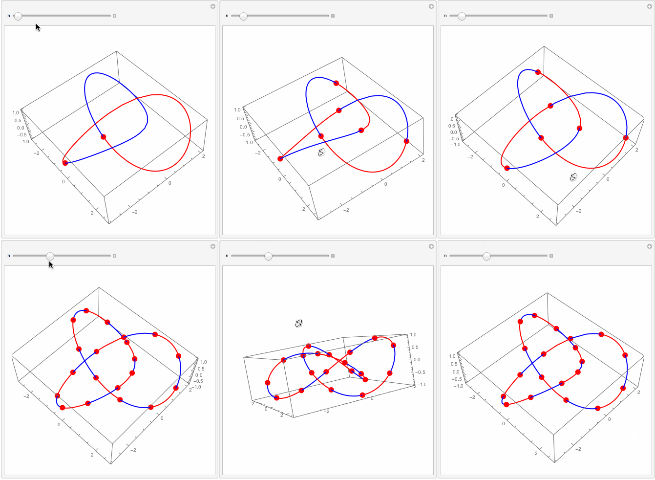
Just wanted to update everyone that things are much simpler, - there is built in support for this:

MeshFunctions -> {"ArcLength"} 

So for our case:

Show[{
  ParametricPlot3D[KnotData[{3, 1}, "SpaceCurve"][t], {t, 0, 2 Pi},

   (* the trick *)
   Mesh -> 15,
   MeshFunctions -> {"ArcLength"},

   (* styles *)
   MeshStyle -> Directive[Red, PointSize[.03]],
   MeshShading -> {Red, Blue}],

  (* the boundary split point *)      
  Graphics3D[{Red, PointSize[.03], 
    Point[KnotData[{3, 1}, "SpaceCurve"][0]]}]}]

Answer 3

Here's one way to implement Yves's suggestion:

(* arclength function *)
trefarc = \[FormalS] /. First[NDSolve[
          {\[FormalS]'[t] == Norm[KnotData[{3, 1}, "SpaceCurve"]'[t]], \[FormalS][0] == 0},
           \[FormalS], {t, 0, 2 Pi}, Method -> "Extrapolation"]]

(* length of trefoil *)
end = trefarc[2 Pi];

With[{n = 25}, (* n - number of points to generate *)
     pts = (KnotData[{3, 1}, "SpaceCurve"][\[FormalT]] /. 
           FindRoot[trefarc[\[FormalT]] == #,
           {\[FormalT], Rescale[#, {0, end}, {0, 2 Pi}], 0, 2 Pi}]) & /@
           (end*Range[0, 1, 1/n])]

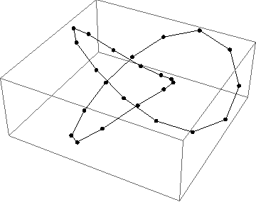
Graphics3D[{Line[pts], AbsolutePointSize[6], Point /@ pts}]

---

In case the code given above was not sufficiently transparent to readers:

1. The arclength function trefarc is produced through the use of Mathematica's numerical differential equation solver NDSolve[] (thus yielding an InterpolatingFunction[] suitable for evaluation); recall that the function $s(t)=\int_0^t g(u)\;\mathrm du$ is the solution to the initial value problem $s^\prime(t)=g(t)$, where $g(t)$ is the norm of the derivative of your (plane or space) curve with respect to the parameter.

2. We can use FindRoot[] for inverting monotonically increasing functions like the arclength function $s(t)$. I used the bracketed form of FindRoot[], FindRoot[eqn, {var, start, min, max}] to ensure that the algorithms within FindRoot[] do not go outside the domain of the InterpolatingFunction[]. For the starting point, since the arclength function looks almost like a line, I used Rescale[] to produce the inverse function of the line joining $(0,0)$ and $(2\pi,s(2\pi))$.

---

Taking a page from Szabolcs's code, the snippet for generating pts can be shortened a fair bit:

With[{n = 25}, 
 pts = Composition[KnotData[{3, 1}, "SpaceCurve"], 
    InverseFunction[trefarc]] /@ (end*Range[0, 1, 1/n])]

This hinges on the fact that the InterpolatingFunction[] output by NDSolve[] can be inverted by InverseFunction[].

Answer 4

Minimalist:

k[t_]   := KnotData[{3, 1}, "SpaceCurve"][t];
len[r_] := N@Integrate[Total[D[k[t], t]^2], {t, 0, r}];
pts[n_] := Solve[len[t1] == len[2 Pi] #/n, t1, Reals] & /@ Range[n + 1];

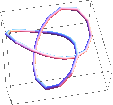
Graphics3D@Tube[k[t1] /. # & /@ (Flatten@pts@30), .1]

Answer 5

This numerical approach is based on length of chord (not arc), so it is a good approximation as long as the curve is smooth and you have close points. You have a parametric curve f of variable t. Define a numerical function that given ti finds such tf that Norm[f[tf]-f[ti]] stays constant. You need 2 functions to keep both negative and positive roots which will show different directions of going arond the knot and will draw knot's different halves.

falMax[ti_] := Max[t /. NSolve[Norm[KnotData[{3, 1}, "SpaceCurve"][t] - 
        KnotData[{3, 1}, "SpaceCurve"][ti]] == .2, t]] // Quiet

falMin[ti_] := Min[t /. NSolve[Norm[KnotData[{3, 1}, "SpaceCurve"][t] - 
        KnotData[{3, 1}, "SpaceCurve"][ti]] == .2, t]] // Quiet

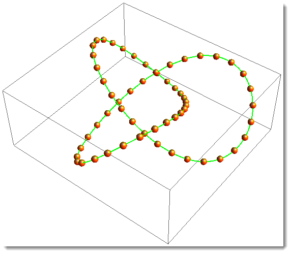
Now the only thing you need is to nest that function - recursively feed it its own output, so it goes in even steps around the knot. Amount of nesting steps you get approximately after a few tries. You do not want to over-draw the extra steps.

Show[Graphics3D[{Orange, Specularity[White, 20], 

   Sphere[#, .1] & /@ (KnotData[{3, 1}, "SpaceCurve"] /@ 
      NestList[falMax[.5], 0, 30]), 

   {Sphere[#, .1] & /@ (KnotData[{3, 1}, "SpaceCurve"] /@ 
       NestList[falMin[.5], 0, 30])}}], 

ParametricPlot3D[KnotData[{3, 1}, "SpaceCurve"][t], {t, 0, 2 Pi}, 
  PlotStyle -> Directive[Green, Thick]]]

Answer 6

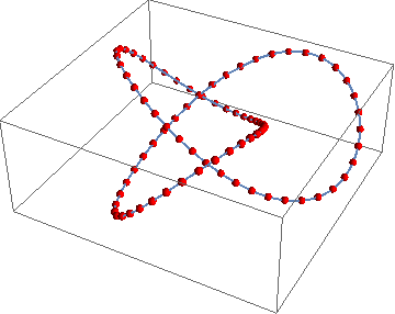
Here is another way to get points equally spaced by chord-length. It will give a good result if the chord length is relatively small compared to the maximum radius of curvature along the curve. (If, say, the chord length is no greater than the maximum radius, then between successive points, the turning will be less 60 deg., and the difference between the chord and arc lengths will be less than 5%).

The method is fast because the objective function, which is the sum of the squares of the differences in the lengths of adjacent chords, is quick to be minimized (provided the initial values are ordered). Another reason is that the speed of this particular parametrization does not vary much, which leads to excellent initial points.

The first and last point are set equal to the end points of the curve. The code below assumes that the parametrization is periodic. The end points are assumed to be equal and one of them is discarded.

xFN = KnotData[{3, 1}, "SpaceCurve"];
nPts = 80;                                                (* number of points *)

Block[{t},
 t[1] = 0; t[nPts + 1] = 2 Pi;                            (* initialize end points *)
 sols = Array[t, nPts] /. 
   Last@FindMinimum[
     Total[Differences[Norm /@ Differences[xFN /@ Array[t, nPts + 1]]]^2], 
     Table[{t[i], (i - 1)/(nPts) 2 Pi}, {i, 2, nPts}]];   (* omit end points *)
 ]

Show[
 Graphics3D[{Red, Translate[Sphere[{0, 0, 0}, 0.08], xFN /@ sols]}],
 ParametricPlot3D[xFN[t], {t, 0, 2 Pi}]
 ]

P.S. If you desire relatively few points so that the chord length is greater than the radius of curvature, then generate many points and down-sample. To get the 80 points above took slightly over 1/20 sec. One can get 8 equally spaced points from the above calculation by using sols[[;; ;; 10]]:

Show[Graphics3D[{Red, Translate[Sphere[{0, 0, 0}, 0.08], xFN /@ sols[[;; ;; 10]]]}], 
 ParametricPlot3D[xFN[t], {t, 0, 2 Pi}]]