DynamicModule issues with Refresh, double evaluation, and CDF Player preview

Question

I am in the middle of making a CDF for a calculation of many random variables. I've gone with DynamicModule and have read the documentation plus these posts: 32294 and 30079. I've obviously missed a few things as it is not working as expected.

I have constructed the module as such (working snippet at the end of post):

DynamicModule[
 {dynamic variables},
 constant variables;
 Dynamic@Refresh[
  expensive calcs;
  plots and tables;
, TrackedSymbols->{update}]

Column[{controls for dynamic variables, plots, tables}],

Initialization :> (functions for calcs, plots, and controls),

UnsavedVariables :> {update},
SaveDefinitions -> True
]

I am having 4 issues.

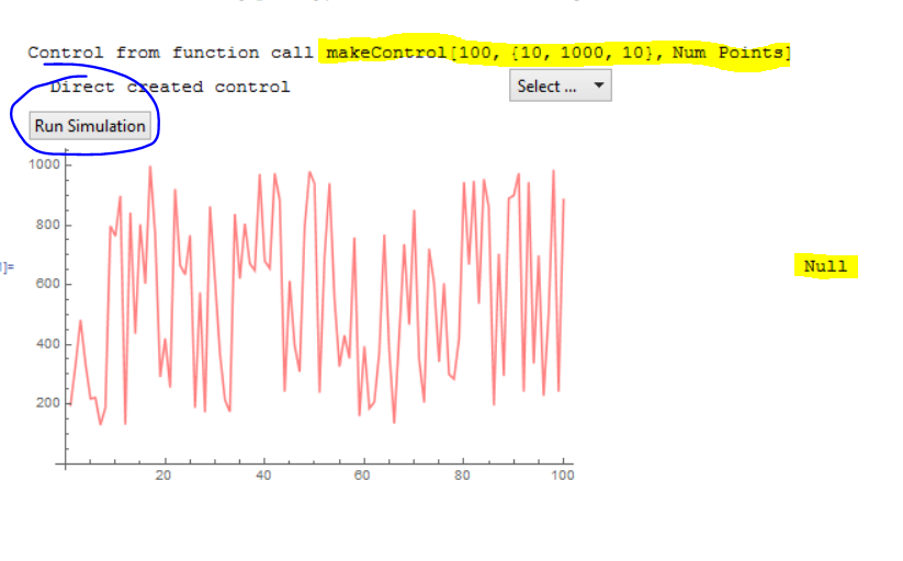
1. The controls created by the makeControl function (variableRow in the larger example) for the dynamic variables do not display on first execution but everything else does. That is, if you

   • delete the output cell,
   • quit and then start the kernel,
   • and execute the module

   then those controls show as the text of the commands that make them. Then executing the module a second time the controls show as the are supposed to.

   The plots and charts are linked to the update variable and refresh when the Run Simulation button is clicked on both the first evaluation and the second evaluation.

2. The Dynamic@Refresh keeps kicking out a Null. If I end it with a ; then none of the plots and tables update when the Run Simulation button is pressed. This seems odd that making it not display output makes it not run the code inside. How do I get rid of this Null? Is this a bug?

3. When previewed as CDF Player I get a ton of errors from the FE' context when I click the Run Simulation button. I have SaveDefinitions -> True on the module so am not certain why this is happening.

4. When the CDF Player is previewed moving the window it is in causes the simulation to repeatedly run. This only happens until the Run Simulation button is pressed. After it is pressed moving the window does not cause the simulation to run. It is an expensive simulation so this behaviour is very much not desired.

---

• First execution with previous output deleted and kernel quit and restart. Direct created controls (the popup and button) work and update the plot when as expected. The control created with makeControl is not available.
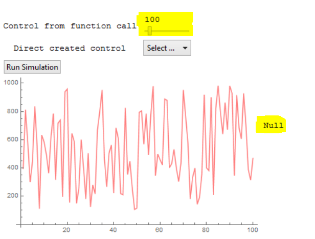
• Second execution immediately after first. The control created with makeControl is now available and updates the plot as expected with the other controls.
• FE' context errors from CDF Player preview.

---

Added a smaller example of issue

This has the same four problems described above.

DynamicModule[
 {numPoints = 100, interpolation = None, update = 1},

 plotColour = Pink;
 Dynamic@Refresh[
    data = RandomReal[{100, 1000}, numPoints];
    plot = plotPoints[data, plotColour, interpolation];
    ,
    TrackedSymbols -> {update}]

   Column[{
    Grid[{
      {"Control from function call", 
       makeControl[Dynamic@numPoints, {10, 1000, 10}, "Num Points"]},
      {"Direct created control", 
       PopupMenu[Dynamic@interpolation, Range[5], "Select ..."]}
      }],
    Button["Run Simulation", update = update + 1, ImageSize -> Large],
    Dynamic@plot
    }]
 ,
 Initialization :>
  (
   plotPoints[points_, colour_, interpOrder_] := 
    ListLinePlot[points, PlotStyle -> colour, 
     InterpolationOrder -> interpOrder, ImageSize -> 400];

   makeControl[variable_, range_, name_] :=
    Column[{variable,
      Slider[variable, range, Appearance -> Tiny, ImageSize -> Tiny]
      }];
   ),
 UnsavedVariables :> {update}, SaveDefinitions -> True]

---

Orignal code snippet (too large and busy). Use simpler example above.

It is a big module so I've taken a lot of things out while preserving my issue. The functions definitions have been reduced as well so please don't focus on the calculations.

DynamicModule[
 (* Parameters *)
 {numberOfRuns = 10000,
  investmentCaptial = 15000000,
  (* Many more dynamic parameters in this section *)
  μOverheadExpenses = 600000, σOverheadExpenses = 40000,
  μReturnOnInvest = 0.05, σSpliceLower = 
   0.03, σSpliceUpper = 0.02,
  update = 1},

 rtnPeriods = {50, 100, 250, 500, 1000};
 variableNames = {(* 
   more names for the omitted dynamic variables above *) 
   "OverheadExpenses", "ReturnOnInvestLogN", "ReturnOnInvestSpliceN"};
 (* A few other constant parameters in this section *)

 Dynamic@Refresh[
    (* Many distributions defined in this section to the dynamic parameters omitted above *)
    overheadExpensesDist = 
     NormalDistribution[μOverheadExpenses, σOverheadExpenses];
    returnOnInvestLogNDist = 
     LogNormalDistribution[1 + μReturnOnInvest, 
      Sqrt[σSpliceLower^2 + σSpliceUpper^2]];
    returnOnInvestSpliceNDist = 
     SplicedDistribution[{σSpliceLower/σSpliceUpper, 
       1}, {-∞, μReturnOnInvest, ∞}, { 
       NormalDistribution[μReturnOnInvest, σSpliceLower], 
       NormalDistribution[μReturnOnInvest, σSpliceUpper]}];

    (* Single step simulation *)

    sampleRuns = 
     Transpose[
      RandomVariate[#, numberOfRuns] & /@ {(* 
        More distributions here o the dynamic parameters omitted above *)
        overheadExpensesDist, returnOnInvestLogNDist, 
        returnOnInvestSpliceNDist}];

    runsAssoc = AssociationThread[variableNames, #] & /@ sampleRuns;

    (* Calculations begin *)
    {netIncomeInvestLogN, netIncomeInvestSpliceN} = 
     Transpose[(Function[{rtnOnInvest}, 
           netIncome[(* 
            More dynamic parameter names here *)#OverheadExpenses,

            Switch[rtnOnInvest, "ReturnOnInvestLogN", 
             Log[#[rtnOnInvest]] - 1, 
             "ReturnOnInvestSpliceN", #[rtnOnInvest]],
            investmentCaptial]] /@ {"ReturnOnInvestLogN", 
           "ReturnOnInvestSpliceN"}) & /@ runsAssoc];

    {netIncomeDistPlotLogN, 
      netIncomeDistPlotSpliceN} = {distributionPlot[
       netIncomeInvestLogN, 
       PlotLabel -> 
        "Investment Return \[Distributed] " <> 
         ToString@Head[returnOnInvestLogNDist], ImageSize -> 400], 
      distributionPlot[netIncomeInvestSpliceN, 
       PlotLabel -> 
        "Investment Return \[Distributed] " <> 
         ToString@Head[returnOnInvestSpliceNDist], ImageSize -> 400]};

    {netIncomeInvestLogNHdt, netIncomeInvestSpliceNHdt} = 
     DistributionFitTest[#, NormalDistribution[x, y], 
        "HypothesisTestData"] & /@ {netIncomeInvestLogN, 
       netIncomeInvestSpliceN};

    {netIncomeInvestLogNReturnPeriod, 
      netIncomeInvestSpliceNReturnPeriod} = 
     returnPeriodTables[{netIncomeInvestLogNHdt, 
       netIncomeInvestSpliceNHdt}, "Net Income"];

    (* More calcuations, tables, and plots on simulation *)
    ,
    TrackedSymbols -> {update}
    ]

  Column[{
    Grid[{
      {, "Distribution", "Mean", "Std. Deviation"},
      (* More variable rows here *)
      Evaluate@
       variableRow["Overhead Expense", "Normal", 
        Dynamic@μOverheadExpenses, {500000, 4000000, 25000}, 
        Dynamic@σOverheadExpenses, {30000, 100000, 5000}],

      {Item["Return On Investment", Alignment -> Center], "Log Normal",
       Item[
        Column[{Dynamic@μReturnOnInvest,

          Slider[Dynamic@μReturnOnInvest, {.01, .08, .005}, 
           Appearance -> Tiny, ImageSize -> Tiny]}, 
         Alignment -> {Center, Center}],
        Alignment -> Center],
       Item[
        Dynamic@Sqrt[σSpliceLower^2 + σSpliceUpper^2], 
        Alignment -> {Center, Bottom}]},
      {SpanFromAbove, "Splice Normal", SpanFromAbove,
       Row[{
         Column[{Dynamic@σSpliceLower,

           Slider[Dynamic@σSpliceLower, {.001, .1, .001}, 
            Appearance -> Tiny, ImageSize -> Tiny]}, 
          Alignment -> {Center, Center}],
         Column[{Dynamic@σSpliceUpper,

           Slider[Dynamic@σSpliceUpper, {.001, .1, .001}, 
            Appearance -> Tiny, ImageSize -> Tiny]}, 
          Alignment -> {Center, Center}]
         }, Spacer[2]]},

      {, "Number of Runs", 
       PopupMenu[Dynamic[numberOfRuns], Range[25000, 100000, 25000], 
        "Select ..."]}


      }],
    Button["Run Simulation", update = update + 1, ImageSize -> Large],


    Dynamic@netIncomeDistPlotLogN,
    Dynamic@netIncomeInvestLogNReturnPeriod
    }, Dividers -> {None, {-3 -> True}}]

 ,
 (* Initialise functions *)
 Initialization :>
  (
   netIncome[(* parameters removed for example *)overheadExpenses_, 
     returnOnInvestment_, investmentCapital_] :=
    returnOnInvestment*investmentCapital - overheadExpenses;

   distributionPlot[data_List, 
     opts : OptionsPattern[{Histogram, SmoothHistogram}]] :=
    With[{μ = Mean@data, σ = StandardDeviation@data},
     Show[
      Histogram[data, 30, "PDF", 
       Sequence @@ FilterRules[{opts}, Options[Histogram]], 
       Frame -> {{False, False}, {True, False}}],
      SmoothHistogram[data, 
       Sequence @@ FilterRules[{opts}, Options[SmoothHistogram]]]
      ]];

   returnPeriodTables[hypoTestData_List, valueHeading_String] := 
    TableForm[
       Transpose@{Function[{rp}, 
           AccountingForm[InverseCDF[#["FittedDistribution"], 1/rp](*,
            DigitBlock\[Rule]{3,2}*)]] /@ rtnPeriods, rtnPeriods}, 
       TableHeadings -> {None, {valueHeading, "Return Period"}}] & /@ 
     hypoTestData;

   variableRow[name_String, 
     distributionName_String, μVariable_, μVariableRange_, σVariable_, σVariableRange_] :=
    {name, distributionName,
     Column[{μVariable,
       Slider[μVariable, μVariableRange, Appearance -> Tiny, 
        ImageSize -> Tiny]}, Alignment -> {Center, Center}],
     Column[{σVariable,
       Slider[σVariable, σVariableRange, 
        Appearance -> Tiny, ImageSize -> Tiny]}, 
      Alignment -> {Center, Center}]};
   ),
 UnsavedVariables :> {update},
 SaveDefinitions -> True
 ]

Answer 1

Edit I've updated my answer entirely since the updated question

First Issue

As detailed in the documentation for Initialization, this expression is not evaluated until after the content of the DynamicModule has been evaluated and not until "the construct is first displayed". This requires that any Initialization variable must be wrapped in Dynamic to be displayed in the DynamicModule output. As a minimal example, see here:

DynamicModule[{localV},
 Grid[{{Slider[Dynamic@localV], 
    function[Dynamic[localV], "Hello World"], globalV}}],
 Initialization :> (function[a_, b_] := {b, a}; globalV = 33)]

Wrapping the entirety of the Grid in Dynamic fixes that:

DynamicModule[{localV},
 Dynamic@Grid[{{Slider[Dynamic@localV], 
     function[Dynamic[localV], "Hello World"], globalV}}],
 Initialization :> (function[a_, b_] := {b, a}; globalV = 33)]

Wrapping Dynamic around makeControl[Dynamic@numPoints...] in your code will fix this issue.

Second Issue

I cannot explain why your example actually works in the absence of the CompoundExpression (;), but I can explain how to use Refesh in the way you would like.

Refresh only affects the Dynamic it is local to, not the entire DynamicModule interface. See the following example below. Note the necessity to include x;y for y to be updated, as detailed in the excellent answer from @MichaelE2 here: https://mathematica.stackexchange.com/a/21643/1952.

DynamicModule[{x, y}, Column[{
   Slider[Dynamic[x]], Slider[Dynamic[y]],
   {"x", Dynamic[x]},
   {"unlimited y", Dynamic[y]},
   {"limited y", Dynamic@Refresh[x; y, TrackedSymbols :> {x}]}
   }]]

Your example can therefore be fixed by expanding the Dynamic owning your Refresh to the entire first argument of the DynamicModule

DynamicModule[
 {numPoints = 100, interpolation = None, update = 1},

 plotColour = Pink;
 Dynamic@Refresh[
    data = RandomReal[{100, 1000}, numPoints];
    plot = plotPoints[data, plotColour, interpolation];
    ,
    TrackedSymbols -> {update}]

   Column[{
    Grid[{
      {"Control from function call", 
       makeControl[Dynamic@numPoints, {10, 1000, 10}, "Num Points"]},
      {"Direct created control", 
       PopupMenu[Dynamic@interpolation, Range[5], "Select ..."]}
      }],
    Button["Run Simulation", update = update + 1, ImageSize -> Large],
    Dynamic@plot
    }]
 ,
 Initialization :>
  (initialisationstuff),
 UnsavedVariables :> {update}, SaveDefinitions -> True]

Third Issue

While you do have SaveDefinitions->True you do have UnsavedVariables, if this is removed your example will work perfectly on my machine.

Fourth Issue

Turns out that there is an issue with PlotTheme potentially making Dynamic visualisations sensitive to window movements, as identified by @SquareOne here https://mathematica.stackexchange.com/a/75489/1952