12
$\begingroup$

I have searched other threads, but I was not successful in finding an answer I could understand.

Right to the point: how do I impose correctly periodic behavior on the edges of the rectangular region without knowing what the behavior is (using FEM in Mathematica)?

Minimal problem in 2D:

I am beginning to work with the new FEM in Mathematica 10 and I am interested in solving problems in pure space (no time, or just stationary if you want) with periodic space conditions for the unknown field in a rectangular regions. I am trying to solve the following minimal problem, but there is something I am missing and I dont get what.

Needs["NDSolve`FEM`"]
reg = ImplicitRegion[0 < 1, {{x1, 0, 1}, {x2, 0, 1}}];
eq0 = -Laplacian[u[x1, x2], {x1, x2}] - 10 x1^5*x2^3;
ucorner = 0;
(*
uedgex1 = (x1 - 1/2)^2 - 1/4;
uedgex2 = (x2 - 1/2)^2 - 1/4;
*)
conds = {
(*corners*)
DirichletCondition[u[x1, x2] == ucorner, x1 == 0 && x2 == 0]
, DirichletCondition[u[x1, x2] == ucorner, x1 == 1 && x2 == 0]
, DirichletCondition[u[x1, x2] == ucorner, x1 == 0 && x2 == 1]
, DirichletCondition[u[x1, x2] == ucorner, x1 == 1 && x2 == 1]
};
(*edges*)
(*
, DirichletCondition[u[x1, x2] == uedgex1, 0 < x1 < 1 && x2 == 0]
, DirichletCondition[u[x1, x2] == uedgex1, 0 < x1 < 1 && x2 == 1]
, DirichletCondition[u[x1, x2] == uedgex2, x1 == 0 && 0 < x2 < 1]
, DirichletCondition[u[x1, x2] == uedgex2, x1 == 1 && 0 < x2 < 1]
*)
ufem = NDSolveValue[{eq0 == 0, conds}, u, Element[{x1, x2},reg]];
Plot3D[ufem[x1, x2], Element[{x1, x2},reg], PlotRange -> All, AxesLabel -> {x1, x2}]

If you solve the problem imposing the behavior on the edges, of course you will get this and the solution is periodic in x1 and x2 (u[0,x2] = u[1,x2] for all x2, corresponding edge behavior is identical, but I just impose it).
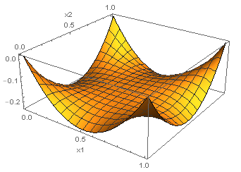
Solution with imposed edge behavior

Without imposing anything on the edges you will get this solution (of course not periodic in x1 or x2, u[x1,0] != u[x1,1] for all x1 and u[0,x2] != u[1,x2] for all x2)
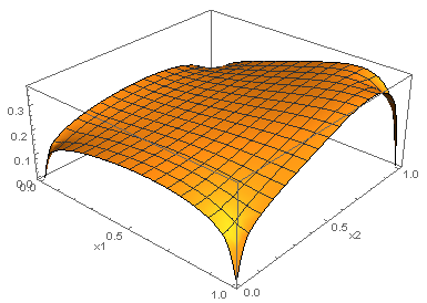
Solution with free edges

Again my question: how do I impose correctly periodic behavior on the edges of the rectangular region without knowing what the behavior is (using FEM in Mathematica)? I have tried to impose the Dirichlet conditions like

DirichletCondition[u[x1, x2] == u[x1, 0], x2 == 1]

but they are not accepted. What am I missing? Thank you very much for an answer, the correct working code or any link to where I cam find my mistake. Greets

Mauricio

EDIT 1:

Thank you user21, I took a look into the documentation (its really awesome!!) and until now I have understood the following:

(*Obtain FEM state*)
{state} = NDSolve`ProcessEquations[{eq0 == 0, conds}, u, Element[{x1, x2}, nr], Method -> {"FiniteElement", "MeshOptions" -> {"MaxCellMeasure" -> 0.2}, "InterpolationOrder" -> {u -> 2}, "IntegrationOrder" -> 2}];
femstate = state["FiniteElementData"];
(********************************************)
(*Set everything manually*)
(*Unknown field, numerical region and mesh*)
vd = NDSolve`VariableData[{"DependentVariable" -> {u}, "Space" -> {x1, x2}}];
nr = ToNumericalRegion[Rectangle[{0, 0}, {1, 1}]];
mesh = ToElementMesh[nr, "MaxCellMeasure" -> 0.2];
plmesh = Show[mesh["Wireframe"["MeshElement" -> "MeshElements","MeshElementIDStyle" -> Blue, "ContinuousElementID" -> True]],mesh["Wireframe"["MeshElement" -> "PointElements","MeshElementIDStyle" -> Red]]];
(*Solution data*)
sd = NDSolve`SolutionData[{"Space" -> nr}];
(*Settings*)
methodData = InitializePDEMethodData[vd, sd, Method -> {"FiniteElement", "InterpolationOrder" -> {u -> 2}, "IntegrationOrder" -> 2}]
(*Initialize PDE coeffs, BCs, discretize system and get system matrices*)
initCoeff = femstate["PDECoefficientData"];
initBCs = InitializeBoundaryConditions[vd, sd, {conds}];
discretePDE = DiscretizePDE[initCoeff, methodData, sd];
stiffness = discretePDE["StiffnessMatrix"];
load = discretePDE["LoadVector"];
discreteBCs = DiscretizeBoundaryConditions[initBCs, methodData, sd];
DeployBoundaryConditions[{load, stiffness}, discreteBCs]
(*Solution, interpolation function and plot*)
solution = LinearSolve[stiffness, load];
uif = ElementMeshInterpolation[{mesh}, solution];
plsol = Plot3D[uif[x1, x2], {x1, x2} \[Element] mesh];
GraphicsRow[{plmesh,plsol}]
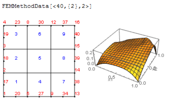
Output 1

All commands are very clear but my last problem now is how to extract in an elegant form the node numbers on the edges without the corners (value on the corners imposed in Dirichlet conditions) and directly connect the corresponding nodes on the opposite edge. Until now I have used the following awful code, but I cannot think of anything smarter at the moment (it's 5 am :D). Any thoughts? (I mean, later I will try to use this for 3D rectangles and my approach is of course the most horrible way to do it). After that I would use the Lagrange multipliers as you explained.

mcoo = mesh["Coordinates"];
belnum = mesh["BoundaryElements"][[1, 1]] //Flatten //DeleteDuplicates;
belinfo = Table[{belnum[[i]], mcoo[[belnum[[i]]]]}, {i, Length[belnum]}];
(*Get corner nodes*)
c00 = Position[belinfo[[;; , 2]], {0., 0.}][[1, 1]];
n00 = belinfo[[c00, 1]];
c01 = Position[belinfo[[;; , 2]], {0., 1.}][[1, 1]];
n01 = belinfo[[c01, 1]];
c10 = Position[belinfo[[;; , 2]], {1., 0.}][[1, 1]];
n10 = belinfo[[c10, 1]];
c11 = Position[belinfo[[;; , 2]], {1., 1.}][[1, 1]];
n11 = belinfo[[c11, 1]];
Print["Corner nodes"]
ncs = {n00, n01, n10, n11}
(*Get first nodes on edge with x1=0 without corner nodes*)
infopos = Position[belinfo[[;; , 2, 1]], 0.] // Flatten;
edgex10 = belinfo[[infopos, 1]];
Do[edgex10 = DeleteCases[edgex10, ncs[[i]]], {i, Length[ncs]}]
Print["Edge with x1=0 without corner nodes"]
edgex10
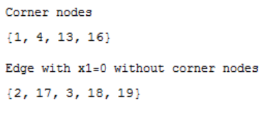
Output 2

$\endgroup$
4
  • $\begingroup$ sorry to see no response here -- I suspect you are pushing past the capability of the "new in 10" FEM capability. $\endgroup$
    – george2079
    Commented Jan 14, 2015 at 23:24
  • 1
    $\begingroup$ Unfortunately, this is not possible out of the box in V10. With some programming one could write some code that does this. How difficult that is depends on two things: Do you always have rectangular domains and are you always looking at stationary problems? The real problem is that I do not have the time to do if for you :-( $\endgroup$
    – user21
    Commented Jan 15, 2015 at 10:08
  • 1
    $\begingroup$ @george2079 : really? That's kind of sad, I was really excited about the new FEM. $\endgroup$ Commented Jan 16, 2015 at 7:48
  • $\begingroup$ @user21 : yes, I always want to take a look at stationary problems in rectangular regions. What are your thougts, just in principle? $\endgroup$ Commented Jan 16, 2015 at 8:48

2 Answers 2

9
$\begingroup$

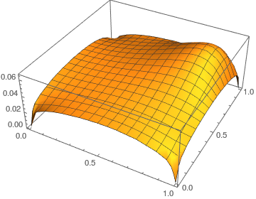
Version 11.0 has an additional boundary condition PeriodicBoundaryCondition. With this you can then use:

ufun = NDSolveValue[{-Laplacian[u[x, y], {x, y}] == 10 x^5*y^3,
    DirichletCondition[u[x, y] == 0, x == 0 && y == 0], 
    PeriodicBoundaryCondition[u[x, y], 0 <= y <= 1 && x == 1, 
     FindGeometricTransform[{{0, 0}, {0, 1}}, {{1, 0}, {1, 1}}][[2]]],
     PeriodicBoundaryCondition[u[x, y], 0 <= x <= 1 && y == 1, 
     FindGeometricTransform[{{0, 0}, {1, 0}}, {{0, 1}, {1, 1}}][[
      2]]]}, u, {x, y} \[Element] Rectangle[{0, 0}, {1, 1}]];

Plot3D[ufun[x, y], {x, y} \[Element] Rectangle[{0, 0}, {1, 1}]]

This also works on non-rectangular regions. One thing to be aware of is that you only need one DirichletCondition since that is mapped to the opposite side and the by now two conditions are mapped to the other opposite side making them four all in all.

enter image description here

$\endgroup$
4
  • 4
    $\begingroup$ Dude, dont take this personally.. but I love you!! :D Thanks a lot!! Does this also work for 3D problems? I just have my phone and can not test anything at the moment. $\endgroup$ Commented Aug 8, 2016 at 18:57
  • 1
    $\begingroup$ Yes, works in 3D for time dependent with variable coefficients etc... You may also send positive feedback to the support ;-) I hope it does not disappoint. $\endgroup$
    – user21
    Commented Aug 8, 2016 at 18:59
  • 1
    $\begingroup$ @MauricioLobos, I think I am going to print this comment - you know, for bad days... $\endgroup$
    – user21
    Commented Aug 8, 2016 at 20:17
  • 2
    $\begingroup$ Hahahaha sure! Your constant support is very appreciated, I really mean that for you and everybody in this great community who just help others just because it is nice! This kind of place and the people here just make the world better! Thanks to all! $\endgroup$ Commented Aug 8, 2016 at 22:25
17
$\begingroup$

Too long for a comment:

OK, first set up your system that you only have non periodic BCs. Then look at the Finite Element programming tutorial and use NDSolve ProcessEquations and follow the steps until the call to DiscretizePDE and DiscretizeBoundaryConditions. At this point you can extract the system matrices. Deploy the (non periodic) boundary conditions. Until here everything is documented.

Periodic boundary conditions come in pairs; an algebraic constraint it added to the system of equations.

Here is an example: Create a system matrix and a load vector:

n = 5;
matrix = Table[ 
   Switch[ j - i, -1, 1, 0, -2, 1, 1, _, 0], {i, n}, {j, n} ];
loadVector = Table[ i, { i, n } ];

Now, for example, we would like to change the system equations such that u1 == u3. We do this with Lagrangian multipliers:

lv = ConstantArray[0, {n}];
(* set u1-u3, for example *)
lv[[1]] = 1;
lv[[3]] = -1;

(* add lagrange row *)
matrix2 = Join[matrix, {lv}];
(* add lagrange col *)
matrix3 = Join[matrix2, Partition[Join[lv, {0}], 1], 2]

(*
{{-2, 1, 0, 0, 0, 1}, {1, -2, 1, 0, 0, 0}, {0, 1, -2, 1, 0, -1}, {0, 
  0, 1, -2, 1, 0}, {0, 0, 0, 1, -2, 0}, {1, 0, -1, 0, 0, 0}}
*)

The system is now larger because we added the equation u1 - u3 and we need to enlarge the load vector as well; we want the the equation u1 - u3 == 0

(* set u1-u3 == 0 *)
load2 = Join[loadVector, {0}];

Solve the equations:

res = LinearSolve[matrix3, load2]
{-(31/4), -(35/4), -(31/4), -(19/2), -(29/4), -(23/4)}

And check that u1 == u3

res[[{1, 3}]]
{-(31/4), -(31/4)}

Hope this helps.

OK, after the update, here is how I'd do it:

reg = Rectangle[{0, 0}, {1, 1}];
(*Obtain FEM state*)
{state} = 
  NDSolve`ProcessEquations[{eq0 == 0, conds}, u, 
   Element[{x1, x2}, reg], 
   Method -> {"FiniteElement", 
     "MeshOptions" -> {"MaxCellMeasure" -> 0.2, "MeshOrder" -> 1}, 
     "IntegrationOrder" -> 2}];
femstate = state["FiniteElementData"];
methodData = femstate["FEMMethodData"];
initBCs = femstate["BoundaryConditionData"];
initCoeff = femstate["PDECoefficientData"];
sd = state["SolutionData"][[1]];
discretePDE = DiscretizePDE[initCoeff, methodData, sd];
stiffness = discretePDE["StiffnessMatrix"];
load = discretePDE["LoadVector"];
discreteBCs = DiscretizeBoundaryConditions[initBCs, methodData, sd];
DeployBoundaryConditions[{load, stiffness}, discreteBCs]

So far so good. The "InterpolationOrder" setting you used is to be able specify different interpolation order for coupled systems, which we do not have here. So the interpolation order will always be the same as the mesh order. Also, we extract everything from the state data. That may be a bit more convenient then to set this up manually. But by all means do as you like.

Extract and visualize the mesh:

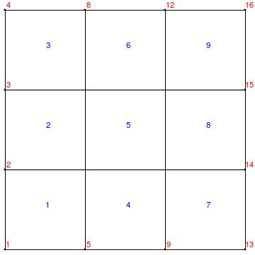
mesh = NDSolve`SolutionDataComponent[sd, "Space"]["ElementMesh"];
Show[
 mesh["Wireframe"["MeshElementIDStyle" -> Blue]]
 , mesh["Wireframe"["MeshElement" -> "PointElements", 
   "MeshElementIDStyle" -> Red]]]

enter image description here

Now, we extract the positions of the relevant coordinates:

c = mesh["Coordinates"];
cornerPos = Position[c, Alternatives @@ Tuples[{0., 1.}, 2]];
tc = Transpose[c];
zeroPos = Position[tc[[1]], 0.]
onePos = Position[tc[[1]], 1.]
(*
{{1}, {2}, {3}, {4}}
{{13}, {14}, {15}, {16}}
*)

left = Flatten[Complement[zeroPos, cornerPos]]
right = Flatten[Complement[onePos, cornerPos]]
(*
{2, 3}
{14, 15}
*)

We use the left nodes as master nodes and the right nodes as slave nodes.

dof = methodData["DegreesOfFreedom"];
lmdof = Length[left];

Now, we are going to hack a bit. This is not documented. We are going to create a DiscretizedBoundaryConditionData that we can then use in DeployBoundaryConditions. This is a bit risky as the internal data structure may change in the future. (You may want to wrap this in a function and if the data structure changes then you'd only need to fix it in that function and not everywhere where you used the code.)

We create a matrix where positions in every row are set to +1 and -1 as explained above.

diriMat = SparseArray[{}, {lmdof, dof}];
MapThread[(diriMat[[#1, #2]] = {1, -1}) &, {Range[lmdof], 
   Transpose[{left, right}]}];

Specify where we have Dirichlet rows:

diriRows = left;

Specify the Dirichlet values which are zero in our case:

diriVals = SparseArray[{}, {lmdof, 1}];

We create the DiscretizedBoundaryConditionData data structure:

lmDiscrete = 
  DiscretizedBoundaryConditionData[{SparseArray[{}, {dof, 1}], 
    SparseArray[{}, {dof, dof}], diriMat, diriRows, 
    diriVals, {dof, 0, lmdof}}, 1];

The first sparse array (which is zero) is added to the load, the second (which is also zero in our case) is added to the stiffness matrix. Then diriMat, diriRows and diriVals are specified. Last some size parameters are given. (What I'll need to think about is to provide an interface to generate DiscretizedBoundaryConditionData such that such hacks are not requited.)

DeployBoundaryConditions[{load, stiffness}, lmDiscrete, 
 "ConstraintMethod" -> "Append"]
(*Solution,interpolation function and plot*)
solution = LinearSolve[stiffness, load];
(* Truncate solution back to dof size *)
solution = Take[solution, dof];

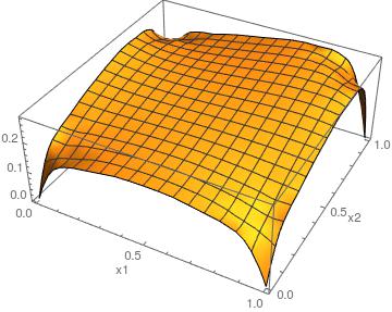
When you crank up "MeshOptions" -> {"MaxCellMeasure" -> 0.02, "MeshOrder" -> 2} you get something like this:

uif = ElementMeshInterpolation[{mesh}, solution];
Plot3D[uif[x1, x2], Element[{x1, x2}, reg], PlotRange -> All, 
 AxesLabel -> {x1, x2}]

enter image description here

And

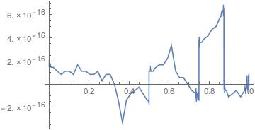
Plot[uif[0, y] - uif[1, y], {y, 0, 1}]

All good? ;-)

enter image description here

$\endgroup$
7
  • $\begingroup$ Thank you very much for the thoughts and the very clear example! I am not a hero in programming but I will give it a shot after having read the documentation you referred to. $\endgroup$ Commented Jan 16, 2015 at 14:17
  • $\begingroup$ @MauricioLobos, were you able to get this to work? $\endgroup$
    – user21
    Commented Jan 19, 2015 at 8:57
  • $\begingroup$ I have not tried it until now (sadly I have some other urgent work to do at the moment), I am still reading the documentation you pointed at. I need to understand this completly, since I want to use it for 3D problems (homogenization of mechanical properties of 3D microstrucutres for problems with periodic boundary conditions). I hope I can solve it this week, but that depend on the urgent thing. Thanks again for the thoughts and sorry for the delay. $\endgroup$ Commented Jan 20, 2015 at 9:29
  • $\begingroup$ @MauricioLobos, just let me know if you have trouble solving it. $\endgroup$
    – user21
    Commented Jan 20, 2015 at 9:39
  • $\begingroup$ Hey user21, if you have some time, could you take a look at the EDIT 1 of the question? The documentation was awesome, but I have some problems in extracting the nodes on the boundary. $\endgroup$ Commented Jan 25, 2015 at 4:19

Your Answer

By clicking “Post Your Answer”, you agree to our terms of service and acknowledge you have read our privacy policy.

Not the answer you're looking for? Browse other questions tagged or ask your own question.