How to plot an implicit value funtion

Question

Previous question has been solved (Gap in a continuous plot). Here is a new related question.

dist = MixtureDistribution[{6, 4}, {NormalDistribution[1, 0.3], 
       NormalDistribution[3, 0.3]}]

f[x_, y_] := y InverseSurvivalFunction[dist, x + y]

Given function f[x,y], for any x, we can get the optimal value y*[x] to maximize f[x,y]. Notice: for some range of x, there are two local maximums for the function and we should select the global one. My question is how to plot y*[x] on support [0,1].

The following codes may help you better understand what y*[x] looks like (decreasing-> jumping up-> decreasing):

Manipulate[
 Plot[y InverseSurvivalFunction[dist, x + y], {y, 0, 1}, 
  ImageSize -> 400, PlotRange -> {{0, 1}, {-1, 2}}], {x, 0, 1}]

Plot3D[y InverseSurvivalFunction[dist, x + y], {y, 0, 1}, {x, 0, .5}, 
 ImageSize -> 400, PlotRange -> {0, 1}]

Answer 1

Plot the objective function f[x,y] for 100 values of x:

plt = Plot[ y InverseSurvivalFunction[dist, # + y] & /@ Range[0, 1., .01], {y, 0, 1},
         Evaluated -> True, ImageSize -> 400, PlotRange -> {{0, 1}, {-.1, 1}}];

Post-proces the previous plot to mark points corresponding to the global maximum on each of the 100 curves:

plt /. Line[x_] :> {Line[x], Red, PointSize[Medium], 
                    Point[Select[x, #[[2]] >= Max[x[[All, 2]]] &]]}

Get the points corresponding to global maxima:

ystarlist = Cases[plt, Line[x_] :> Select[x, #[[2]] >= Max[x[[All, 2]]] &][[1]], {0, Infinity}];

ListPlot[ystarlist[[All, 1]], Frame -> True, Joined -> True, 
 DataRange -> {0, 1},
 PlotRange -> {{0, 1}, {0, 1}}, AspectRatio -> 1, PlotStyle -> Thick, 
 FrameLabel -> (Style[#, 16, "Panel"] & /@ {"x", "ystar(x)"})]

Update: Using NArgMax (much slower than the above method):

ystarlist2 =  NArgMax[{y InverseCDF[dist, 1 - # - y], 0. < y <= 1. - #}, y,
    Method -> {"SimulatedAnnealing", "PerturbationScale" -> 3,
      "BoltzmannExponent" -> Function[{i, df, f0}, -df/(Exp[i/10])]}] & /@ Range[0., .99, .01]

ListPlot[ystarlist2 , Joined -> True, Frame -> True, DataRange -> {0, 1}, 
 PlotRange -> {0, 1}, AspectRatio -> 1,
 PlotStyle -> Thick, FrameLabel -> (Style[#, 16, "Panel"] & /@ {"x", "ystar(x)"})]

Update 2:

how to add the mirror image relative to 45 degree line

ListPlot[{d1 = MapIndexed[{#2[[1]]/100, #} &, ystarlist[[All,1]]], Reverse /@ d1}, 
 Joined -> {True, True}, PlotStyle -> {Directive[Thick, Red], Directive[Thick, Blue]}, 
 Frame -> True, PlotRange -> {0, 1}, AspectRatio -> 1,
 FrameLabel -> (Style[#, 16, "Panel"] & /@ {"x, BR(y)", "y, BR(x)"}),
 PlotLegends -> LineLegend[{Style["BR(x)", 16, "Panel"], Style["BR(y)", 16, "Panel"]}]]

Answer 2

First some analysis. The slowness is due to the time it takes to compute InverseSurvivalFunction[dist, u]. InverseSurvivalFunction is a general purpose function and perhaps not optimized for mixture of normal distributions. An improvement in speed can be obtained by using some calculus to reduce the number of times we have to compute InverseSurvivalFunction. Another problem is that InverseSurvivalFunction cannot be differentiated in Mathematica. We can again use some calculus to derive formulas for its derivatives. In this approach we will use NDSolve to calculate approximations. These should be fairly accurate, but if high precision is needed, one will have to adapt the NDSolve code or switch back to using InverseSurvivalFunction directly and put up with the slowness. It may be possible to use NIntegrate, which usually can compute integrals more accurately than NDSolve, but that may be what InverseSurvivalFunction is doing anyway.

Preliminary analysis and outline of solution

Let sf and isf stand for the survival function and inverse survival function, respectively, of our distribution dist. The derivatives of isf may be written in terms of the derivatives of sf and the undifferentiated isf:

D[InverseFunction[sf][u], u]
D[%, u]

Since the derivative of sf has a nice expression,

dsf[w_] = D[SurvivalFunction[dist, w], w]
(*  -(2/3) E^(-(50/9) (-3 + w)^2) Sqrt[2/π] - E^(-(50/9) (-1 + w)^2) Sqrt[2/π]  *)

we will be able use it to make more easily computed derivatives of isf with rules like the following (these will be adapted to our final code later, but I will need them in the present discussion):

derivatives = {
  isf[u_] :> InverseSurvivalFunction[dist, u],
  Derivative[1][isf][u_] :> 1/dsf[InverseSurvivalFunction[dist, u]],
  Derivative[2][isf][u_] :> -dsf'[InverseSurvivalFunction[dist, u]] /
    dsf[InverseSurvivalFunction[dist, u]]^3
  }

For a given value of x, one condition for a maximum of y isf[x + y] is

D[y isf[x + y], y] == 0
(*  isf[x + y] + y Derivative[1][isf][x + y] == 0  *)

Once we find such a maximum, its rate of change as x is governed by the differential equation

D[D[y isf[x + y], y] == 0 /. y -> y[x], x]
(*
  Derivative[1][isf][x + y[x]] Derivative[1][y][x] + 
    Derivative[1][isf][x + y[x]] (1 + Derivative[1][y][x]) + 
    y[x] (1 + Derivative[1][y][x]) Derivative[2][isf][x + y[x]] == 0
*)

where the first and second derivatives of isf are given by the formulas in derivatives above. We can find initial local maxima for, say, x == 1/4, with FindMaximum by choosing convenient starting points. Note we have to supply a derivative (via the Gradient option) for Newton's method to work. Otherwise, FindMaximum will choose a non-gradient method, which will skip around more and will not always find the nearest local maximum.

FindMaximum[y InverseSurvivalFunction[dist, x + y] /. x -> 1/4, {y, y0}, 
 Method -> "Newton", 
 Gradient -> {D[y isf[x + y], y] /. x -> 1/4 /. derivatives}]

We can determine the starting points by simply plotting y isf[dist, 1/4 + y], or quickly scanning a table of values for sign changes of the derivative from plus to minus:

With[{signs = Sign@Table[D[y isf[x + y], y] /. x -> 1/4 /. derivatives // Evaluate,
                         {y, 0.01, 0.7, 0.01}]},
 Most @ Accumulate[
    Length /@ (Split[signs] //.
        {a___, n : {__?Negative}, p : {__?Positive},  b___} :> {a, Join[n, p], b})
  ]/100.
 ]
(*  {0.14, 0.57} *)

Feeding these to FindMaximum will yield the two distinct local maxima mentioned by the OP.

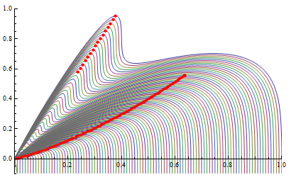
Once we have the two starting points we can solve the differential equation above. It will yield two solutions for y[x], each of which will trace the trajectory of a local maximum of y isf[x + y] as x varies. Simply choosing the Max of these two at each x gives the y★[x] function sought by the OP.

Implementation

For the above to work quickly, we need a way to quickly evaluate isf. That is our first step. It is done by integrating the derivative of the InverseSurvivalFunction. This leads to the differential equation

isf'[u] == 1/dsf[isf[u]]

We need an initial condition, for which I chose a value for u very close to zero:

isf[SurvivalFunction[dist, 10]] == 10

Note that due to the nature of an inverse function, we do not even have to evaluate InverseSurvivalFunction once here.

Clear[isf]
dist = MixtureDistribution[{6, 4}, {NormalDistribution[1, 3/10], NormalDistribution[3, 3/10]}];
dsf[w_] = D[SurvivalFunction[dist, w], w];
nisf = NDSolveValue[
    {isf'[u] == 1/dsf[isf[u]], isf[SurvivalFunction[dist, 10]] == 10},
    isf,
    {u, SurvivalFunction[dist, 10], SurvivalFunction[dist, 0]}
    ]; // AbsoluteTiming
(*  {0.019727, Null}  *)

In addition to the formulas in derivatives above (and repeated below), we will need numeric versions of them that use nisf above. They, in nderivatives, should be used instead derivatives for speed. In particular we will use them in the differential equation in previous section that gives us the local maxima as a function of x. It will take this form:

yeqn = Numerator[D[D[y isf[x + y], y] /. y -> y[x], x] /. nderivatives // Together] == 0

It is sometimes nice to get rid of denominators in an equation. (Computer sometimes do not like fractions, just like people, although for numerical reasons.) Using our starting points {0.14, 0.57}, we will find the local maxima and store them in ics. These will each serve as an initial condition for each trajectory of the local maxima. One might notice I used derivatives in the Gradient; it is because nderivatives produced a warning that I thought likely would contribute to error in the final result.

nderivatives = {
   isf[u_] :> nisf[u],
   Derivative[1][isf][u_] :> 1/dsf[nisf[u]],
   Derivative[2][isf][u_] :> -dsf'[nisf[u]]/dsf[nisf[u]]^3};
derivatives = {
   isf[u_] :> InverseSurvivalFunction[dist, u],
   Derivative[1][isf][u_] :> 1/dsf[InverseSurvivalFunction[dist, u]],
   Derivative[2][isf][u_] :> -dsf'[InverseSurvivalFunction[dist, u]]/
     dsf[InverseSurvivalFunction[dist, u]]^3};

yeqn = Numerator[D[D[y isf[x + y], y] /. y -> y[x], x] /. nderivatives // Together] == 0;

ics = y /. 
     Last@FindMaximum[
       y InverseSurvivalFunction[dist, x + y] /. x -> 1/4, {y, #}, 
       Method -> "Newton", 
       Gradient -> {D[y isf[x + y], y] /. x -> 1/4 /. derivatives}] & /@ {0.14, 0.57};

{ysol1, ysol2} = NDSolveValue[
      {yeqn, y[1/4] == #},
      y,
      {x, SurvivalFunction[dist, 10], SurvivalFunction[dist, 0]},
      "ExtrapolationHandler" -> {Indeterminate &, "WarningMessage" -> True}
      ] & /@ ics; // AbsoluteTiming

NDSolveValue::ndsz: At x == 0.38987189832043223`, step size is effectively zero; singularity or stiff system suspected. >>

{0.163722, Null}

We get a warning NDSolveValue::ndsz which could be the end of the natural domain of one of the functions. It turns out not to matter. The integration has gone far enough that we can construct the function y★ sought by the OP. So I just ignored the message.

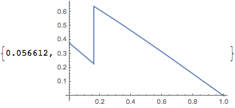
One way to get the function sought by the OP is to use MaximalBy to pick which of the functions ysol1 or ysol2 is greater at each x:

Plot[MaximalBy[{ysol1[x], ysol2[x]} /. 
    Indeterminate -> 1, # nisf[x + #] &], {x, 0, 1}] // AbsoluteTiming

Another way is to construct a piecewise function, in which we have already determined when each function is the maximum.

x0 = x /. 
   FindRoot[
    ysol1[x] nisf[x + ysol1[x]] == ysol2[x] nisf[x + ysol2[x]], {x, 
     0.2}];
y★[x_] = 
 With[{yfns = SortBy[{ysol1, ysol2}, #[0.01] &]},
  Piecewise[{
    {yfns[[1]][x], 
     Simplify[
      Less @@ Insert[Flatten[yfns[[1]]["Domain"]], x, 2] && x < x0]},
    {yfns[[2]][x], 
     Less @@ Insert[Flatten[yfns[[2]]["Domain"]], x, 2]}
    },
   Indeterminate]
  ]

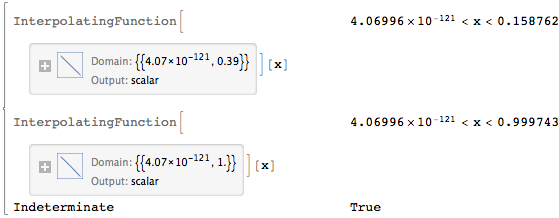
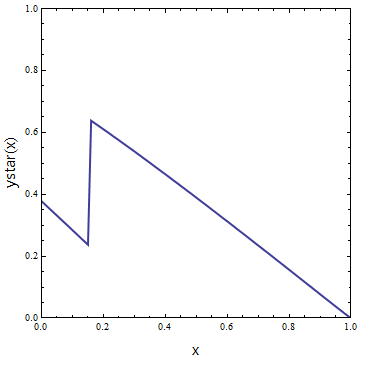
Plot[y★[x], {x, 0, 1}] // AbsoluteTiming

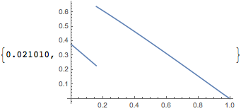
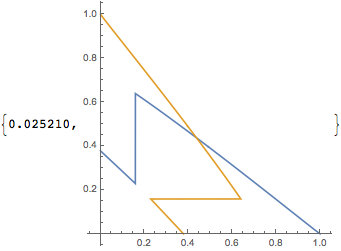
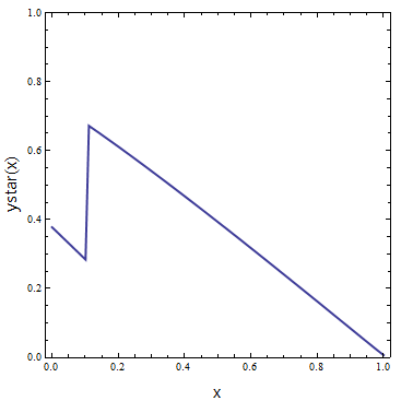
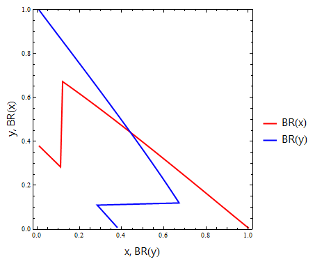
Note that with a Piecewise function Plot does not connect the discontinuity. This might or might not be desired. If not, one can add the option Exclusions -> None. It appears from a comment that the OP is interested in plotting the function y★ and its reflection. Here is a way, with the segments of each graph joined because of Exclusions -> None; omit it if the segments should be disconnected.

ParametricPlot[{{x, y★[x]}, {y★[x], x}},
 {x, 0, 1}, Exclusions -> None] // AbsoluteTiming