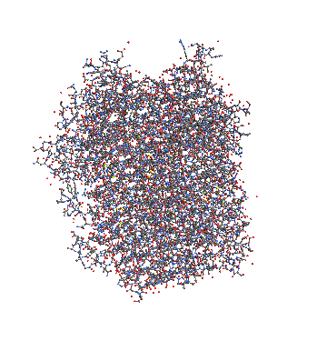
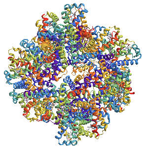
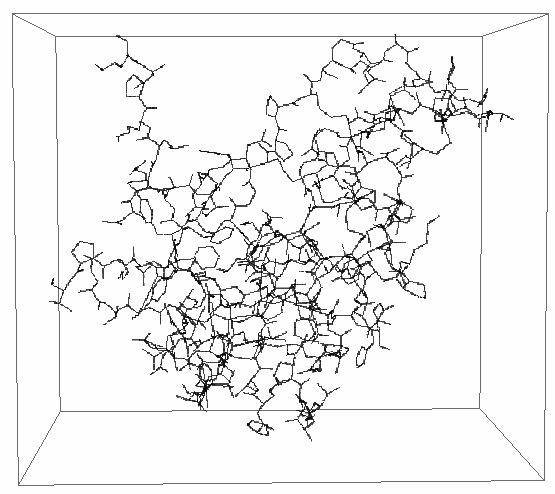
Mathematica should render the secondary structure in the usual way when you import pdb files. I dont know why this doesn't work with the example you provided. I thought there might be a size limit for the protein but I managed to import much bigger proteins such as 1YHU and they got rendered without problems... strange.
Import["http://www.rcsb.org/pdb/download/downloadFile.do?fileFormat=\
    pdb&compression=NO&structureId=1YHU", "PDB"]

I don't know how fractal dimensions of biomolecules are usually calculated but simple box counting is always an option. The box counting dimension of an image can easily be determined by using ImagePartition as done in this post. The algorithm can easily be applied to 3D images.
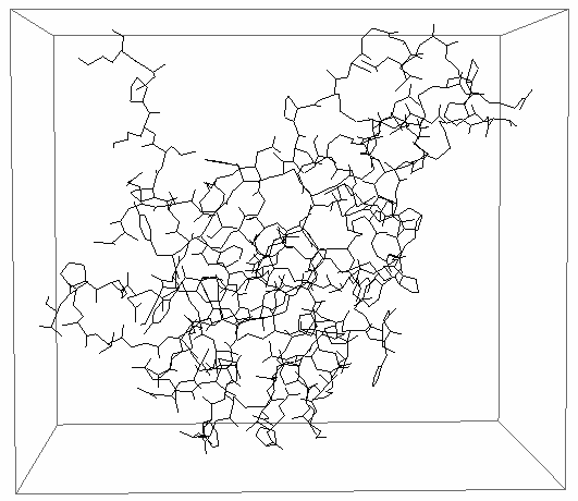
This reduces the problem to the generation of a 3D image from the protein data. I though it was more convinient to use the mol2 format because Mathematica should allow the import of EdgeRules for this format. Anyways, I couldn't get that to work and I ended up extracting the VertexCoordinates and EdgeRules by pattern matching.
data = Import["../2DSP1.mol2", "Lines"];

StringSplit[#] & /@
   StringCases[data, DigitCharacter .. ~~ ___ ~~ "1.000"] //. {} ->
   Sequence[];
coord = ToExpression@Flatten[%, 1][[All, 3 ;; 5]];
StringSplit[#] & /@
   StringCases[data,
    DigitCharacter .. ~~ Whitespace ~~ DigitCharacter .. ~~
     Whitespace ~~ DigitCharacter .. ~~ Whitespace ~~
     DigitCharacter ..] //. {} -> Sequence[];
edgeRules = ToExpression@Rest@Flatten[%, 1][[All, 2 ;; 3]];

Graphics3D[Line[{coord[[#1]], coord[[#2]]}] & @@@ edgeRules]

The conversion to Image3D was done by populating a SparseArray with points along the connection network. This can definitely be improved but you get the idea. The current implementation takes a lot of memory!
ranges = {Floor@Min[#], Ceiling@Max[#]} & /@ Transpose[coord];
scaling = 8;
Image3DDim = scaling (#2 - #1) & @@@ ranges;
lin = LinearSolve[{{ranges[[#, 1]], 1}, {ranges[[#, 2]], 1}}, {1,
      Image3DDim[[#]]}] & /@ Range[3];

raster = 20;
rasterPoints =
  Flatten[Table[
      coord[[#1]] - (coord[[#1]] - coord[[#2]])/raster*a, {a, 0,
       raster}] & @@@ edgeRules, 1];
res = DeleteDuplicates@
   Transpose@
    Flatten[{Round[
         lin[[#, 1]] rasterPoints[[All, #]] + lin[[#, 2]]] & /@
       Range[3]}, 1];

i = Image3D[SparseArray[# -> 1 & /@ res],"Bit",
  ColorFunction -> "WhiteBlackOpacity", Boxed -> True]

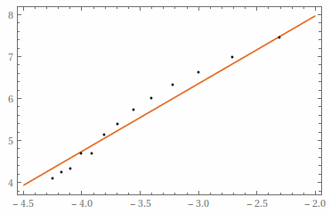
The box counting code gives as a fractal dimension of ~1.6.
MinS = Floor[Min[ImageDimensions[i]]/2];
data = ParallelTable[{1/size,
    Total[Sign /@ (Total[#, 3] & /@ (ImageData /@
          Flatten[ImagePartition[i, size]]))]}, {size, 5, MinS/2, 5}];

line = Fit[Log[data], {1, x}, x]
Plot[line, {x, -4.5, -2}, Epilog -> Point[Log[data]], Frame -> True,
 Axes -> False, PlotTheme -> "Scientific"]
11.2048 + 1.61623 x
