Find $X_t = c_1 X_{t-1} + \dots + c_n X_{t-n} + n_t$ for given $c_i$, initial conditions $(X_1, \dots, X_n)$, and distribution for i.i.d. $n_t$.
I would like to know if there is a more efficient or elegant way to code this than using a for loop.
Find $X_t = c_1 X_{t-1} + \dots + c_n X_{t-n} + n_t$ for given $c_i$, initial conditions $(X_1, \dots, X_n)$, and distribution for i.i.d. $n_t$.
I would like to know if there is a more efficient or elegant way to code this than using a for loop.
Generating an autoregressive time series is not the same as "finding" it, since you have the parameters. If I understand you correctly, this is an application made for FoldList:
Here is a simple AR(1) process to illustrate the technique:
FoldList[c1 #1 + #2&, x0, RandomVariate[NormalDistribution[0,1],{100}]
For example
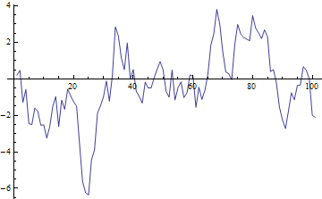
 FoldList[0.9 #1 + #2 &, 0.2, RandomVariate[NormalDistribution[0, 1], {100}]]
 ListLinePlot[%]
For an AR($p$) process with $p>1$, something like this would work:
FoldList[Join[{params.#1+#2},Most[#1]]&, startingvalues,
  RandomVariate[NormalDistribution[0, 1], {100}]]
Where params is your list of c parameters and startingvalues is your list of starting values.
Multivariate processes (i.e. simulation of data from a VAR to get a vector of length $p$ at each time period) can be handled similarly except of course that params will be a matrix and you'll be saving a matrix consisting of the vector of data for the current period, plus the $p$ lags, at each step. Then you need to extract the matrix of data from the repetitions representing the lags at each step using Part, i.e.
FoldList[Join[{matrixofparams.#1+#2},Most[#1]]&, matrixofstartingvalues,
   RandomVariate[NormalDistribution[0, 1], {100,p}]][[All, 1, All ]]
FoldList approach to generating an AR process all the time, to show people how functional programming in Mathematica works, and to generate fake economic-looking data for my test graphs.
$\endgroup$
I like @RM 's approach. Another one, with a more "mathematical" notation (but I must say I'm not certain of the random behaviour of the way I'm getting the numbers) could be the following
First we create the discrete noise
i : noise["Seed"] := i = RandomInteger[{-# , #}] &[Developer`$MaxMachineInteger];
noise[n_Integer] :=
 BlockRandom[SeedRandom[# + n];
    RandomVariate[NormalDistribution[]]] &[noise["Seed"]]
Now, noise is a realisation of the process. You can realise another one by resetting the seed with noise["Seed"]=.;
If you do DiscretePlot[noise[n], {n, 0, 10}] several times, you'll see what I mean.
Now, just use RecurrenceTable
RecurrenceTable[{
    x[0] == 0.5,
    x[1] == 0.54,
    x[2] == -2.3,
    x[n] == noise[n] + 0.75 x[n - 1] - 0.23 x[n - 2] + 0.2 x[n - 3]},
        x[n], {n, 0, 10}]
A straightforward way would be using recursion and memoization. An example:
n = 5;
c = RandomReal[NormalDistribution[], n]/100;

Clear[x]
Array[(x[#] = RandomReal[NormalDistribution[]]) &, n]; (* Initial conditions *)
x[t_Integer] /; t > n := x[t] = c.Table[x[i], {i, t - 1, t - n, -1}] +
     RandomReal[NormalDistribution[]]

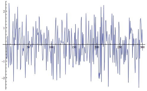
ListLinePlot[x /@ Range[300]]
c.Table? What it does?
$\endgroup$
Commented
Apr 7, 2016 at 17:38
Since Version 9 you can also use the built-in functions RandomFunction and ARProcess:
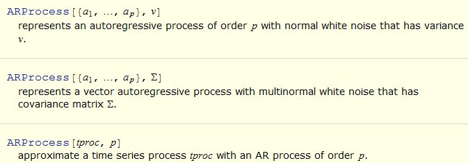
For example, to generate data following an AR(1) process with parameter .3 you can use
SeedRandom[1]
RandomFunction[ARProcess[{.3}, 1], {1, 100}];
ListLinePlot[%]
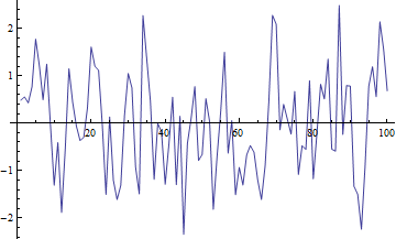
which, except for the initial observation, is identical to the data generated using Verbeia's approach:
SeedRandom[1]
FoldList[0.3 #1 + #2 &, 0, RandomVariate[NormalDistribution[0, 1], {100}]];
ListLinePlot[%]
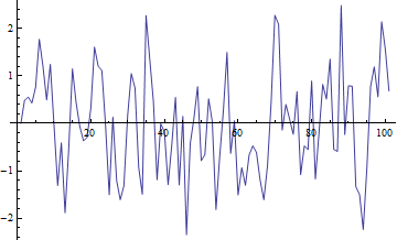
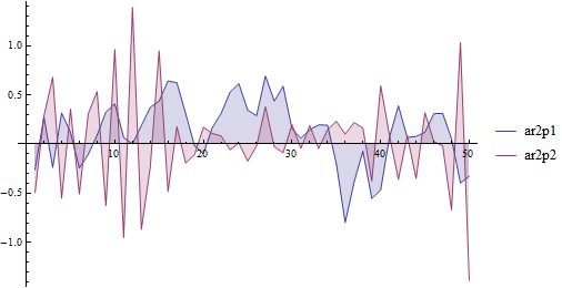
Two AR(2) processes:
ar2p1 = RandomFunction[ARProcess[{0.9, -.3}, .1], {1, 50}];
ar2p2 = RandomFunction[ARProcess[{-0.9, -.3}, .1], {1, 50}];

ListLinePlot[{ar2p1, ar2p2}, Filling -> Axis, PlotLegends -> {"ar2p1", "ar2p2"}]
