How to fix problems solving for values of BSpline function?

Question

I generated a spline function called f using the BSplineFunction with domain {t, 0, 1}.

f = BSplineFunction[{{0., 5.81152}, {-0.909122, 5.73997}, {-1.86805, 5.5031}, 
  {-1.79586, 5.52709}, {-2.40811, 5.28912}, {-3.4109, 4.70527}, {-4.68131,   3.501}, 
  {-4.93131, 2.99958}, {-5.09697, 2.6673}, {-5.34697, 2.16588}, {-5.59697, 1.66446}, 
  {-5.84697, 1.16304}}, SplineWeights -> {10, 10, 10, 1, 1, 1, 1, 1, 1, 10, 10, 10}]

I then wanted to find the points at which the function intersects the piecewise linear function joining the spline's control points. Graphically, I know the intersection occurs within the domain of f.

k[t_] = {-4.93131 - 0.915666 t, 2.99958 - 1.83654 t}

However, running the code:

FindRoot[First[k[0]] == First[f[t]], {t, .5, 0, 1}]

where k[0] is the end of the line, produces a negative number. Is there a way to solve for the intersection points of those two functions?

Answer 1

This is yet another problem that can be solved by explicitly representing the B-spline curve with BSplineBasis[], as was done here:

pts = {{1, 1}, {2, 3}, {3, -1}, {4, 1}, {5, 0}};

(* piecewise linear interpolant *)
lin = Interpolation[pts, InterpolationOrder -> 1];

n = Min[Length[pts] - 1, 3]; (* B-spline degree *)
m = Length[pts];
(* clamped uniform knots for B-spline *)
knots = {ConstantArray[0, n + 1], Range[m - n - 1]/(m - n),
         ConstantArray[1, n + 1]} // Flatten;

{xu, yu} = Transpose[pts];

(* B-spline component functions *)
bf[t_] = xu.Table[BSplineBasis[{n, knots}, i - 1, t], {i, Length[pts]}];
bg[t_] = yu.Table[BSplineBasis[{n, knots}, i - 1, t], {i, Length[pts]}];

From here we use a trick similar to what was done in this answer; use the MeshFunctions option of Plot[] to find initial estimates for the intersection, and then polish those estimates with FindRoot[]:

crs = Cases[Normal[Plot[bg[t] - lin[bf[t]], {t, 0, 1},
                        Mesh -> {{0}}, MeshFunctions -> {#2 &}]], 
            Point[{x_, _}] :> (Through[{bf, bg}[\[FormalT]]] /. 
                               FindRoot[bg[\[FormalT]] - lin[bf[\[FormalT]]],
                                        {\[FormalT], x}]), ∞]
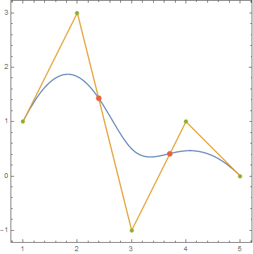
   {{2.3914022076831603, 1.4343911692673563}, {3.707060176019142, 0.4141203520382841}}

Visualize the geometry:

ParametricPlot[{bf[t], bg[t]}, {t, 0, 1}, 
               Epilog -> {{Directive[AbsoluteThickness[1.6], ColorData[97, 2]], 
                           Line[pts]},
                          {Directive[AbsolutePointSize[6], ColorData[97, 3]], 
                           Point[pts]},
                          {Directive[AbsolutePointSize[8], ColorData[97, 4]], 
                           Point[crs]}},
               PlotRange -> {Automatic, {-1, 3}}, PlotRangePadding -> Scaled[.05]]

Answer 2

Clear["Global`*"]
pts = {{1, 1}, {2, 3}, {3, -1}, {4, 1}, {5, 0}};
f1 = Interpolation[pts, InterpolationOrder -> 1];
f2 = BSplineFunction[pts];
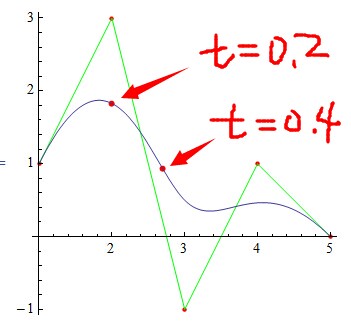
Show[Graphics[{Red, Point[pts], PointSize[0.02], 
   Point[f2 /@ {0.2, 0.4}], Green, Line[pts]}, Axes -> True], 
   ParametricPlot[f2[t], {t, 0, 1}]]

First,determine approximate range of t, in my example tmin = 0.2, tmax = 0.4.

Then,use method of dichotomy to find the point we need.

dichotomy[{t1_, t2_}] :=
 Module[{x1, x2, y1, y2, tmid, x3, y3},
  {x1, x2} = First@f2[#] & /@ {t1, t2};
  {y1, y2} = f1 /@ {x1, x2};
  tmid = (t1 + t2)/2;
  {x3, y3} = f2[tmid];
  If[(y1 - Last@f2@t1)*(f1[x3] - Last@f2@tmid) < 0, {t1, tmid}, {tmid, t2}]
  ]
tmin = 0.2; tmax = 0.4; error = 10^-5.;
ans = First@NestWhile[dichotomy, {0.2, 0.4}, 
     With[{p = f2@First@#}, f1@First@p - Last@p > error] &]

0.306755

Last, check the answer:

f2[ans]
f1@First@f2[ans]

{2.3914, 1.4344}

1.4344

Answer 3

Define the spline for numerical values only and solve for x and y coordinate simultaneously.

g[t_?NumericQ] = f[t]

fr = FindRoot[{First[k[0]], a} == g[t], {t, .7}, {a, 1}]

(*   {t -> 0.674177, a -> 2.99958}   *)

{f[t], k[0]} /. fr

(*   {{-4.93131, 2.99958}, {-4.93131, 2.99958}}   *)

Answer 4

Since V10, one can use Indexed[.., 1] instead of First[..] or Part:

FindRoot[Indexed[k[0], 1] == Indexed[f[t], 1], {t, .5, 0, 1}]
(*  {t -> 0.674177}  *)