Marking the points of x-intercept on a plot

Question

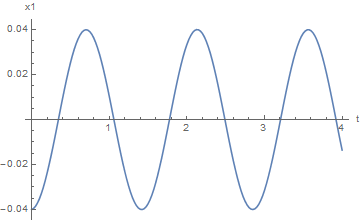
OK, I have a nice plot of some oscillating motion. I can read some stuff off the graph, but I thought it would be cool to show a dot where the curve hits the x-axis and a little label showing the coordinates, and thus get a direct measure of the period of oscillation. (I know there are equations for that but that's not quite the point of the exercise).

Anyhow, here's the code I am using

Clear[x1, x2, v1, v2];Clear[x1, x2, v1, v2];
ti = 0; tf = 4.; delta = (1/40);
x1[ti] = -0.04; x2[ti] = -0.04; v1[ti] = 0.0; v2[ti] = 0.0;
m1 = 0.1890; m2 = 0.1898; k = 3.65; kc = 3.5;
Do[ F1[t] = -k*x1[t] - kc*(x1[t] - x2[t]); 
 F2[t] = -k*x2[t] - kc*(x2[t] - x1[t]);
 v1[t + delta] = v1[t] + (F1[t]/m1)*delta; 
 v2[t + delta] = v2[t] + (F2[t]/m2)*delta;
x1[t + delta] = x1[t] + v1[t + delta]*delta;    
 x2[t + delta] = x2[t] + v2[t + delta]*delta,
 {t, ti, tf, delta}] 
x1data = Table[{t, x1[t]}, {t, ti, tf, delta}];
x1plot = ListPlot[x1data, AxesLabel -> {"t", "x1"}, Joined -> True]

and with it I get a nice graph:

I tried using NSolve and didn't get any output at all. So I think NSolve must not be geared to this.

Understand I am a rank beginner with Mathematica. So it's ok to assume I am stupid :-) And I know that there are likely more efficient ways to do the curve and such; this is a lab exercise tho. We're testing a simulation against the real data.

Answer 1

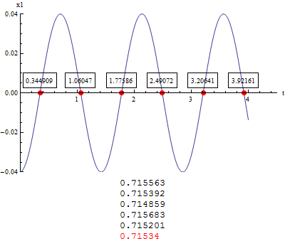
You can display zero crossing using MeshFunctions. Here is a clumsy exploitation from created graphic. The half-periods (difference between consecutive points) are displayed below with mean in red.

x1plot = ListPlot[x1data, AxesLabel -> {"t", "x1"}, Joined -> True, 
  MeshFunctions -> (#2 &), Mesh -> {{0.}}, 
  MeshStyle -> {Red, PointSize[0.02]}];
pts = x1plot[[1, 2, 1]];
me = pts[[First@Cases[x1plot, Point[x_] :> x, Infinity]]];
plt = Column[{ListPlot[x1data, AxesLabel -> {"t", "x1"}, 
    Joined -> True, MeshFunctions -> (#2 &), Mesh -> {{0.}}, 
    MeshStyle -> {Red, PointSize[0.02]}, 
    Epilog -> (Text[Framed[First@#], #, {0, -1.4}] & /@ me), 
    PlotRangePadding -> {{0, 0.5}, {0, 0}}, ImageSize -> 400],
   Column[
    Join[(diff = Differences[me[[All, 1]]]), {Style[Mean@diff, Red]}]]
   }, Alignment -> Center]

Answer 2

To get an output similar to ubpdqn's you can also post-process the output of ListPlot to modify points adding text labels:

modifyF = Normal[#] /. Point[x_] :> {Point[x], Black, 
  Inset[Framed[x[[1]], Background -> Yellow], x, Scaled[{.5, -.2}]]} &;

Examples:

lp = ListPlot[x1data, AxesLabel -> {"t", "x1"}, Joined -> True, 
   MeshFunctions -> (#2 &), Mesh -> {{0.}}, MeshStyle -> {Red, PointSize[0.015]}, 
   PlotRangeClipping -> False, ImageSize -> 400];
Row[{lp, modifyF@lp}, Spacer[10]]

For

x1data2 = Table[100 x Cos[x] Sin[x], {x, -2 Pi, 2 Pi, 4 Pi/100}];

we get