2d heat conduction equation: Boundary and initial conditions are inconsistent

Question

I have the following code for a 2d heat c equation:

 soln = NDSolve[{        D[y[r, f, t], r, r] + 
                   (1/r)*D[y[r, f, t], r] +
                 (1/r^2)*D[y[r, f, t], f, f] == 
                                (1/1.27*10^-4)*D[y[r, f, t], t], 
          y[r, f, 0] == 0, 
          y[10^-2, f, t] == 0,
          (D[y[r, f, t], r] /. 
               r -> 2*10^-6) == -(1/(3.14*10^-8))*(1 + Sin[2*2*3.14*t/2]), 
          (D[y[r, f, t], f] /. f -> 0) == -(10/238)*y[r, 0, t], 
          (D[y[r, f, t], f] /. f -> 3.14/2) == 0}, 
                    y, {r, 2*10^-6, 10^-2}, {f, 0, 3.14/2}, {t, 0, 1}]

and I'm getting the two following error messages:

NDSolve::ibcinc: Warning: Boundary and initial conditions are inconsistent

NDSolve::mxst:Maximim number of 10000 steps reached at the point t==1.629*10^-10

NDSolve::eerr:Scaled local spatial error estimate of 4203.0461 at t=1.840*10^-8 in the direction of independent variable r is much greater than prescribed error tolerance. Grid spacing with 51 points may be too large to achieve the desired accuracy or precision. A singularity may have formed or you may want to specify a smaller grid spacing using the MaxStepSize or MinPoints method options

I saw an answer for the first one so i'm pretty ok with that but the second one is giving me trouble limitting the useful time domain.I cannot figure out why I'm getting this. Any help will be greatly appreciated! Claudiu

Answer 1

Partial answer: the inconsistent boundary condition is that you are specifying df/dr non zero for all t, which is inconsistent with the zero (hence df/dr=0) initial condition.

Ive modified the third condition as:

    (D[y[r, f, t], r] /. 
           r -> 2*10^-6) == -(1/(Pi 10^-8))
                (1 +  Sin[2 Pi t]) Piecewise[{{t 10, t < 1/10  }, {1, True}}]

"ramping up" that BC from zero eliminates the inconsistency warning. However, the solution is still diverging in the corners:

 Plot3D[(y /. soln[[1]])[r, f, 1*^-8] , {r, 2*^-6, 10*^-2}, {f, 0, 
       3.14/2}, PlotRange -> {-100, 1000}]

Answer 2

I'd like to point out OP is probably simulating a point heat source with infinite strength at the center of the circle with the b.c. (D[y[r, f, t], r] /. r -> 2*10^-6) == -(1/(3.14*10^-8))*(1 + Sin[2*2*3.14*t/2]) and this seems to be the most troublesome part of the problem. (To learn more about "point source", check this post. ) I'm not sure about why OP chose this approximation, and guess a better approximation is necessary if one wants to solve the PDE in a not-that-slow way. Anyway, the following is my solution.

First, some clean-up for the equation and parameters, just to make the code more readable:

rrange = {rL, rR} = {2 10^-6, 10^-2};
frange = {fL, fR} = {0, Pi/2};
tbegin = 0;
tend = 1;
eqn = D[y[r, f, t], r, 
     r] + (1/r) D[y[r, f, t], r] + (1/r^2) D[y[r, f, t], f, f] == (100/127 10^-4) D[
     y[r, f, t], t];

ic = y[r, f, tbegin] == 0;
bc = {y[r, f, t] == 0 /. r -> rR, 
   D[y[r, f, t], r] == -((1 + Sin[(2 2 π t)/2])/(π/10^8)) /. r -> rL,
   
   D[y[r, f, t], f] == -(10/238)*y[r, f, t] /. f -> fL, 
   D[y[r, f, t], f] == 0 /. f -> fR};

Then in principle the PDE can be solved with

showStatus[status_] := 
  LinkWrite[$ParentLink, 
   SetNotebookStatusLine[FrontEnd`EvaluationNotebook[], ToString[status]]];
clearStatus[] := showStatus[""];

mol[n_Integer, o_:"Pseudospectral"] := {"MethodOfLines", 
  "SpatialDiscretization" -> {"TensorProductGrid", "MaxPoints" -> n, 
    "MinPoints" -> n, "DifferenceOrder" -> o}}
mol[tf:False|True,sf_:Automatic]:={"MethodOfLines",
"DifferentiateBoundaryConditions"->{tf,"ScaleFactor"->sf}}

soln = NDSolve[{eqn, ic, bc}, y, {r, rL, rR}, {f, fL, fR}, {t, tbegin, tend}, 
    MaxSteps -> Infinity, Method -> Union[mol[True, 100], mol[10, 2]]]; // AbsoluteTiming

Definition of showStatus is from here.

MaxSteps -> Infinity is set to deal with the mxst warning. "DifferentiateBoundaryConditions"->{True,"ScaleFactor"->100} is set to avoid the inconsistent b.c. being severely ignored. (For more information check this post.) "MaxPoints" -> 10, "MinPoints" -> 10, "DifferenceOrder" -> 2 is set to speed up the calculation. According to the monitor, the time step passes 1.840*10^-8 without difficulty, but sadly the calculation is still slow and memory-consuming and my laptop can't bear with it. If you have a PC with more memory, you may have a try, but in the rest part of this answer, I'll decrease the computation burden further by discretizing the PDE to a set of ODE with a coarser grid. (NDSolve won't allow this coarse grid if the PDE is directly sent into NDSolve.)

I'll use the pdetoode function here for discretization.

rpoints = 8;
fpoints = 8;
rgrid =Array[# &, rpoints, rrange];
fgrid = Array[# &, fpoints, frange];
var = Outer[y, rgrid, fgrid];
xdifforder = 2;
torder = 1;
ptoo = pdetoode[y[r, f, t], t, {rgrid, fgrid}, xdifforder];

del = Delete[#, {{1}, {-1}}] &;

odeqn = del /@ del@ptoo@eqn;
odeic = ptoo@ic;
odebc = With[{sf = 100}, diffbc[{t, torder}, sf]@MapAt[del, ptoo@bc, {{1}, {2}}]];

SetAttributes[y, NHoldAll]

clearStatus[]
sollst = NDSolveValue[{odeqn, odeic, odebc} // N, var, {t, tbegin, tend}, 
    Method -> {"EquationSimplification" -> "Solve"}, MaxSteps -> Infinity, 
    EvaluationMonitor :> showStatus["t = " <> ToString[CForm[t]]]]; // AbsoluteTiming
(* {95.391782, Null} *)

sol = rebuild[sollst, {rgrid, fgrid}, 3];

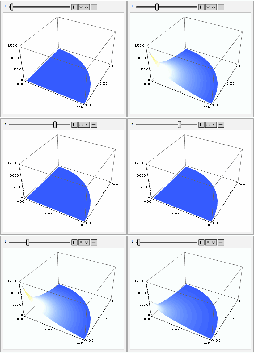
Animate[RevolutionPlot3D[sol[r, f, t], {r, rL, rR}, {f, fL, fR}, 
  PerformanceGoal -> "Quality", ColorFunctionScaling -> False, Mesh -> None, 
  ColorFunction -> (ColorData["TemperatureMap"][#3/(1.5 10^5)] &), 
  PlotRange -> {Automatic, Automatic, {0, 1.5 10^5}}], {t, 0, tend}]

With such a coarse grid, the result still looks not bad: