Why isn't my Stream code plotting multiple solution curves?

Question

My code is:

VectorPlot[
 {1, y*(1 - y) - 0.2  + 0.1*Cos[2*x]}, {x, 0, 15}, {y, 0, 1.2},
 FrameLabel -> {x, y},
 Axes -> True,
 VectorScale -> {Small, Small, None},
 VectorStyle -> Gray,
 StreamPoints -> Coarse,
 StreamStyle -> {Blue, Thin, "Line"},
 StreamScale -> Full
 ]

and my image is

I'd like more than one blue line following my solution curve...

Thanks!

Answer 1

This is not a solution; this is a clue to the nature of the problem. Update: Now there is a solution too; see below.

Consider this very simple streamline plot (note the different bounds on $x$ and $y$):

StreamPlot[{-4 y, x/4}, {x, -1, 1}, {y, -1/4, 1/4}]

In this view the streamlines are all circles, so the ideal plot would just have a lot of evenly spaced circles. Instead Mathematica puts a lot of streamlines at the left and right and very few at the top and bottom. Why? The answer is that it's not trying to make the streamlines be uniformly spaced in the plot, it's trying to make them uniformly spaced in the original $xy$ plane:

StreamPlot[{-4 y, x/4}, {x, -1, 1}, {y, -1/4, 1/4}, AspectRatio -> Automatic]

Check it out: it's exactly the same streamlines. But now the spacing Mathematica has picked looks much more reasonable.

In my opinion, this is totally undesirable behaviour. But, this is we have to work with. So if you want Mathematica to draw a good collection of streamlines that look evenly spaced in the plot, I guess you have to use AspectRatio -> Automatic to make sure that the aspect ratio of the plot matches that of the domain, so that the spacing doesn't get distorted. In your case, this is going to result in an awfully narrow plot. So what you might have to do is rescale the $y$ axis yourself to match the aspect ratio of the plot you want, compute the rescaled vector field, plot it with the modified bounds, and change the ticks on the plot to correspond to the original domain...

---

Here's a simple solution that seems to do the job. We transform the vector field so that the domain is mapped to the unit square $[0,1]\times[0,1]$, create the streamline plot there, and then transform the arrows back to the original domain.

Update 2: Now with variable aspect ratio support! Instead of $[0,1]\times[0,1]$ we'll use the rectangle $[0,1]\times[0,a]$.

Options[myStreamPlot] = Options[StreamPlot];
myStreamPlot[f_, {x_, x0_, x1_}, {y_, y0_, y1_}, opts : OptionsPattern[]] := 
 With[{a = OptionValue[AspectRatio]}, 
  Show[
   StreamPlot[
     {1/(x1 - x0), a/(y1 - y0)} (f /. {x -> x0 + u (x1 - x0), y -> y0 + v/a (y1 - y0)}), 
     {u, 0, 1}, {v, 0, a}, opts]
    /. Arrow[pts_] :> Arrow[({x0, y0} + {x1 - x0, (y1 - y0)/a} #) & /@ pts], 
   PlotRange -> {{x0, x1}, {y0, y1}}]]

So my example works now:

myStreamPlot[{-4 y, x/4}, {x, -1, 1}, {y, -1/4, 1/4}]

Yours takes a little more adjustment.

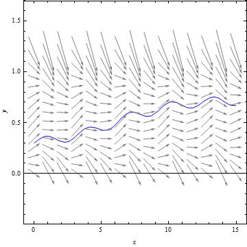
Show[
 VectorPlot[{1, y*(1 - y) - 0.2 + 0.1*Cos[2*x]}, {x, 0, 15}, {y, 0, 1.2},
   FrameLabel -> {x, y}, Axes -> True, VectorScale -> {Small, Small, None}, VectorStyle -> Gray], 
 myStreamPlot[{1, y (1 - y) - 0.2 + 0.1 Cos[2 x]}, {x, 0, 15}, {y, 0, 1.2},
   StreamPoints -> Coarse, StreamStyle -> {Blue, Thickness[Medium]}, StreamScale -> Full, 
   AspectRatio -> 1/2]
  /. Arrow -> Line]