1
$\begingroup$

I have a question. Suposse I have some data with their respective errors:

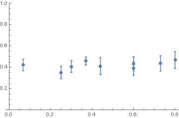
 Data = {{0.067, 0.423}, {0.30, 0.408}, {0.60, 0.433}, {0.25,0.3512}, {0.37, 0.4602}, {0.44, 0.413}, {0.60, 0.390}, {0.73,0.437}, {0.8, 0.47}};


 Errors = {0.055, 0.0552, 0.0662, 0.0583, 0.0378, 0.080, 0.063, 0.072, 0.08};

I want to construct somehow numerical derivatives of these data at som specific point. My idea was first to find a fit of those data (I'm not including the errors so far)

model = a*x + b*x^2 + c*x^3 + d*x^4 + f*x^5 + g*x^6 + h*x^7 + j*x^8 + k*x^9;

fit = FindFit[Dataf, model, {a, b, c, d, f, g, h, j, k}, z];

modelf = Function[{z}, Evaluate[model /. fitfs8]];

fits = Plot[modelf[x], {x, 0, 1.0}, Epilog -> Map[Point, Datafs8], 
 Frame -> True, ImageSize -> 700, PlotStyle -> Directive[Red], 
FrameLabel -> {Style["x", Italic], 
 Style["y", Italic]}, Axes -> False, 
 LabelStyle -> Directive[16]];
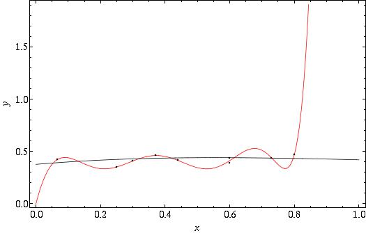
enter image description here

The reason why I choose those model was matter of convenience, since I have some theoretical model (Black line, I don't add the expression because is quite "complicated"). After that I make a Numerical Derivative of the Model and compare with the analytical derivative of the theoretical prediction
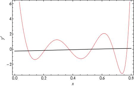
enter image description here

The questions are:

  1. How can I include the errors in the method?
  2. How can I get then expressions (numbers) for y' at some point with errors as well?

I appreciate your help :)

$\endgroup$
2
  • $\begingroup$ You have 18 numbers and 9 errors?? Anyways, with value and error, you could assign in mathematica: number=SetPrecision[value,-Log10[error/value]] $\endgroup$
    – Coolwater
    Commented Jan 30, 2014 at 11:57
  • $\begingroup$ Yes...it.s supossed the data is kind of (x_i,y_i) and errors (Delta y_i) $\endgroup$ Commented Jan 30, 2014 at 13:25

1 Answer 1

2
$\begingroup$

Your data:

data = {{0.067, 0.423}, {0.30, 0.408}, {0.60, 0.433}, {0.25, 0.3512}, {0.37, 0.4602}, {0.44, 0.413}, {0.60, 0.390}, {0.73, 0.437}, {0.8, 0.47}};
errors = {0.055, 0.0552, 0.0662, 0.0583, 0.0378, 0.080, 0.063, 0.072, 0.08};

ErrorListPlot[Transpose[{data, ErrorBar /@ errors}], PlotRange -> {0, 1}]

Mathematica graphics

Assume that the errors are distributed Normally with standard deviation given by your errors. Then we can define

diffErr[y1_, s1_, x1_, y2_, s2_, x2_] := Block[{distr, slope, error},
  distr = 
   TransformedDistribution[(v - u)/(
    x2 - x1), {u \[Distributed] NormalDistribution[y1, s1], 
     v \[Distributed] NormalDistribution[y2, s2]}];
  slope = Mean[distr];
  error = StandardDeviation[distr];
  {slope, error}
  ]

That is the calculation of the slope, provided the vertical values are normally distributed with StdDev given by your errors.

And now the slopes between points ie the numerical derivatives are then

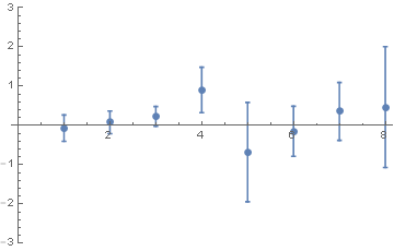
slopes=Table[diffErr[data[[i, 2]], errors[[i]], data[[i, 1]],  data[[i + 1, 2]], errors[[i + 1]], data[[i + 1, 1]]], {i, Length[data] - 1}]
{{-0.0643777, 0.334435}, {0.0833333, 0.287315}, {0.233714, 0.252034}, {0.908333, 0.579016}, {-0.674286, 1.26401}, {-0.14375, 0.636427}, {0.361538, 0.735933}, {0.471429, 1.53756}}
ErrorListPlot[slopes, PlotRange -> {-3, 3}]

Mathematica graphics

$\endgroup$

Your Answer

By clicking “Post Your Answer”, you agree to our terms of service and acknowledge you have read our privacy policy.

Not the answer you're looking for? Browse other questions tagged or ask your own question.