How do I determine the maximum value for a polynomial, given a range of x values?

Question

I need to determine the maximum value for y = a x^2 + b x + c, where I know the coefficients and the upper and lower x values. Say the input values are:

a = 5; b = 1; c = 2; xLower = -5; xUpper  = 5;

Given this input, how do I determine the maximum value for the quadratic function above?

My goal is to implement a function that has a signature such as funcMax[ a, b, c, xUpper, xLower]. How could I get the arguments for the extremal values using the above input?

Answer 1

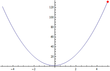
Having an exact input we can find an exact solution:

Maximize[{ 5 x^2 + x + 2, -5 <= x <= 5}, x]

{132, {x -> 5}}

We could simply provide appropriate mathematical tools fulfilling expectations (adequate conditions on derivatives of the function, i.e. vanishing of the first derivative (a critical point) and negativity of the second derivative, then also inspecting boundary values) but with Maximize the task is simplified.

Warning:

Maximize (respectively Minimize) yielding appropriate extremal values of the function can omit some arguments where it has extremal values. This problem can be resolved using Lagrange multipliers (see e.g. How can I implement the method of Langrange multipliers to find constrained extrema?) or solving directly adequate equations.

Example 1

Maximize[{5 x^2 + x + 2, -(26/5) <= x <= 5}, x]

{132, {x -> -(26/5)}}

but recalling the first example we would expect: {132, {x -> -(26/5)}, {x -> 5}}.
To remedy this problem we could do:

Solve[{#1 == First[ Maximize[{#1, #2}, x]], #2}, x]& @@ {     5 x^2 + x + 2, 
                                                          -(26/5) <= x <= 5 }

{{x -> -(26/5)}, {x -> 5}}

Example 2

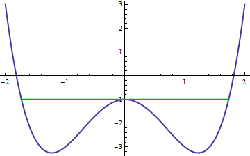
Maximize[{x^4 - 3 x^2 - 1, -Sqrt[3] <= x <= Sqrt[3]}, x]

{-1, {x -> 0}}

Here boundary arguments were omitted, but solving this system we can get all solutions

Union @ 
  Solve[{#1 == First[ Maximize[{#1, #2}, x]], #2}, x]& @@ { x^4 - 3 x^2 - 1,
                                                           -Sqrt[3] <= x <= Sqrt[3]}

 {{x -> 0}, {x -> -Sqrt[3]}, {x -> Sqrt[3]}}

Plot[ x^4 - 3 x^2 - 1, {x, -2, 2}, PlotStyle -> Thick, 
      Epilog -> {Darker @ Green, Thick, Line[{{-Sqrt[3], -1}, {Sqrt[3], -1}}]}]

Similar problems we can encounter in more dimensional spaces and higher order equations.

Answer 2

opt = {a -> 5, b -> 1, c -> 2};
y = a x^2 + b x + c
FindMaxValue[{y /. opt, -5 < x < 5}, x]

(* 131.999999424241 *)

If you want the x value also, use

opt = {a -> 5, b -> 1, c -> 2};
y = a x^2 + b x + c;
r = FindMaximum[{y /. opt, -5 < x < 5}, x];
Plot[y /. opt, {x, -5, 5},Epilog->{Red, PointSize[Large], Point[{x /.Last@r,First@r}]}]

(* {131.999999424241, {x -> 4.9999999887106}} *)

Answer 3

For a quadratic function, sometimes the extreme value (max. or min.) occurs at the vertex, at $x = -b/2a$; otherwise, it will occur at one of the endpoints of the interval.

In this case $a =5 >0$, so the maximum will occur at an endpoint, the one farthest from the vertex, $x = -b/2a = -1/10$. Thus it will be the right endpoint, $x = 5$.

So, in terms of Mathematica, the maximum value is at

a x^2 + b x + c /. {a -> 5, b -> 1, c -> 2} /. x -> 5
(* 132 *)

Or if you would rather evaluate $y$ at both endpoints instead of worrying about which is farthest from the vertex, then

a x^2 + b x + c /. {a -> 5, b -> 1, c -> 2} /. {{x -> -5}, {x -> 5}}
Max[%]

(* {122, 132} *)
(* 132 *)