4
$\begingroup$

I have this set of three data points and I want the natural cubic spline functions for them:

  dat = {{-.0247500, .5}, {.3349375, -.25}, {1.101000, 0}};

I tried:

  f = SplineFit[dat, Cubic]

Using another approach and code, I get the two cubic functions (I am trying to verify the correctness) as:

$$\begin{align*} -0.481347 + 0.753113 x - 0.0338047 x^2 - 0.455282 x^3\\ -0.506486 + 0.978281 x - 0.706073 x^2 + 0.213767 x^3 \end{align*}$$

Is there any way to see these results and the intermediate results to derive the two cubics using Mathematica? (I tried looking at documentation and could not make sense of it.)

$\endgroup$
2
  • $\begingroup$ Are you saying there is no MMA approach to getting the spline points and we have to resort to an interpolating function? $\endgroup$
    – Amzoti
    Commented Nov 5, 2013 at 7:01
  • $\begingroup$ This is a very good question and the answer I believe is no, there is (frustratingly) no direct way to elicit the actual functional form (coefficients) produced by spline fit (or many similar functions) $\endgroup$
    – george2079
    Commented Nov 5, 2013 at 16:09

2 Answers 2

9
$\begingroup$

I've finally decided to write a "modern" re-implementation of the old SplineFit[] routine from NumericalMath`SplineFit`. In the course of writing it, I was struck by how crude it actually is compared to some of the interpolation methods I've presented in past answers. Thus, except for the purpose of reproducing the output of SplineFit[] from old calculations, I do not recommend its use, as there are now better methods.

splinefit[dat_?MatrixQ] :=
          Module[{n = Length[dat], del = Differences[dat]},
                 del = LinearSolve[SparseArray[
                       {Band[{2, 1}] -> 1, 
                        Band[{1, 1}] -> ArrayPad[ConstantArray[4, n - 2], 1, 2], 
                        Band[{1, 2}] -> 1}], 
                       ListCorrelate[{{3}, {3}}, del, {-{1, 1}, {1, 1}}, {0}]];
                 BSplineFunction[#1, SplineDegree -> 3, SplineKnots -> #2] & @@
                 {Join[{dat[[1]]},
                       Riffle[Most[dat] + Most[del]/3, Rest[dat] - Rest[del]/3],
                       {dat[[-1]]}],
                  ArrayPad[Riffle[#, #] &[Range[0, n - 1]], 2, "Fixed"]}]

For instance, here is the example from the old docs:

sf = splinefit[{{0, 0}, {1, 2}, {-1, 3}, {0, 1}, {3, 0}}];

sf[1.4]
   {0.2651428571428573, 2.7017142857142855}

ParametricPlot[sf[t], {t, 0, 4}, AspectRatio -> 1/GoldenRatio]

old SplineFit[] example


Starting with

dat = {{-.0247500, .5}, {.3349375, -.25}, {1.101000, 0}};

use the new splinefit[] on it:

f = splinefit[dat];

Unfortunately, as it stands, BSplineFunction[] objects are immune to exposure from PiecewiseExpand[]. The routine could certainly be modified so that the results are entirely in terms of BSplineBasis[]. Instead, I'll demonstrate some undocumented functionality for extracting knots and control points from BSplineFunction[] objects, which we can then use with BSplineBasis[]:

n = First[f["Degree"]];
knots = First[f["Knots"]];
cpts = f["ControlPoints"];

(A complete(?) list of supported methods can be obtained from f["Methods"].)

The explicit form of the piecewise polynomial functions can then be recovered like so:

fun[x_] = FullSimplify[PiecewiseExpand[
                       Table[BSplineBasis[{n, knots}, j - 1, x],
                             {j, Length[cpts]}].cpts]];

I've omitted the result, but you can compare it yourself with the ones obtained by Ray in his answer.

$\endgroup$
2
  • $\begingroup$ What exactly do you refer to by "there are now better methods"? $\endgroup$
    – murray
    Commented Mar 23, 2019 at 13:57
  • $\begingroup$ @murray: the "natural" spline implemented in the old package is not usually used anymore in applications; one now uses either "not-a-knot" or polynomial fits to get the end conditions needed to produce a unique spline. In addition, the old package uses a uniform parametrization, which is often not the best choice. One can do e.g. centripetal or chord length parametrization to get a better-looking curve. So yes, the old implementation is a little bit long in the tooth. $\endgroup$ Commented Mar 23, 2019 at 14:04
6
$\begingroup$
f1[x_] = a1 + b1*x + c1*x^2 + d1*x^3;
f2[x_] = a2 + b2*x + c2*x^2 + d2*x^3;
s = Solve[{f1 @ dat[[1,1]] == dat[[1,2]],
           f1 @ dat[[2,1]] == dat[[2,2]],
           f2 @ dat[[2,1]] == dat[[2,2]],
           f2 @ dat[[3,1]] == dat[[3,2]],
           f1' @ dat[[2,1]] == f2' @ dat[[2,1]],
           f1'' @ dat[[2,1]] == f2'' @ dat[[2,1]],
           f1'' @ dat[[1,1]] == 0,
           f2'' @ dat[[3,1]] == 0},
          {a1, b1, c1, d1, a2, b2, c2, d2}]
(* {{a1 -> 0.438903, b1 -> -2.46492, c1 -> 0.221098, d1 -> 2.97775,  
     a2 -> 0.603324, b2 -> -3.93762, c2 -> 4.61804, d2 -> -1.39813}} *)
f[x_] = Piecewise[{{f1[x], x ≤ dat[[2, 1]]}}, f2[x]] /. s;

Plot[f[x], {x, dat[[1, 1]], dat[[3, 1]]}, Frame -> True, Axes -> None, 
     Prolog -> {PointSize[.02], Point /@ dat}]
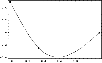
plot

EDIT, Re the comment by @george2079 -- SplineFit uses the same algebra that I used, but instead of fitting y to x, which is what I did, it fits x and y separately to their (zero-based) indices, Range[0, Length @ dat - 1].

( spline = SplineFit[dat, Cubic] ) // InputForm

gives the following, which I have formatted, rounded, and annotated:

SplineFunction[Cubic,
{0., 2.},  (* index range *)
{{-0.02475,    0.5 },  (* x[[1]], y[[1]] *)  
 { 0.3349375, -0.25},  (* x[[2]], y[[2]] *)
 { 1.101,      0   }}, (* x[[3]], y[[3]] *)
{{{-0.02475, 0.25809375, 0., 0.10159375},   (* coeffs for fitting x[[{1,2}]] *)
  { 0.5,    -1.,         0., 0.25      }},  (*   "     "     "    y[[{1,2}]] *)
 {{ 0.3349375, 0.562875, 0.30478125, -0.10159375}, (*  "     "    x[[{2,3}]] *)
  {-0.25,     -0.25,     0.75,       -0.25      }} (*  "     "    y[[{2,3}]] *) }]

There are two splines implicit in the above:

X[u_] = Piecewise[{{-.02475 + .25809375 u + .10159375 u^3, 0 ≤ u ≤ 1},
  {.3349375 + .562875 (u-1) + .30478125 (u-1)^2 - .10159375 (u-1)^3, 1 < u ≤ 2}}];

Y[u_] = Piecewise[{{.5 - u + .25 u^3, 0 ≤ u ≤ 1},
  {-.25 - .25 (u-1) + .75 (u-1)^2 - .25 (u-1)^3, 1 < u ≤ 2}}];

Note that u is shifted so that the argument of the polynomial is always in $[0,1]$.

In the following, changing spline[u] to {X[u], Y[u]} does not change the plot:

ParametricPlot[spline[u],{u, 0, 2}, Frame -> True, Axes -> None,  
               AspectRatio -> Automatic, Prolog -> {PointSize[.02],Point /@ dat}]
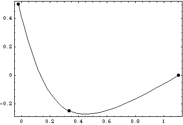
plot

$\endgroup$
2
  • $\begingroup$ note this is a different result from SplineFit. Likely SplineFit uses some different end conditions.. $\endgroup$
    – george2079
    Commented Nov 5, 2013 at 17:22
  • $\begingroup$ InputForm! .. +2 for that if I could.. $\endgroup$
    – george2079
    Commented Nov 6, 2013 at 21:30

Your Answer

By clicking “Post Your Answer”, you agree to our terms of service and acknowledge you have read our privacy policy.

Not the answer you're looking for? Browse other questions tagged or ask your own question.