7
$\begingroup$

How can I produce a fill (in a plot) that extends between two given abscissa values, and "infinitely" in the ordinate direction? (Of course, here "infinitely" just means "up to the top and bottom boundaries of the plot, whatever those may be".)

I thought that RegionPlot would do the trick, but no: RegionPlot requires that the extent of regions be fully specified in both directions; e.g. it does not understand a third parameter having a form anything like {y, -Infinity, Infinity}.

EDIT: Let me clarify the question.

Just as an example, imagine that I have a random bunch of Graphics objects displayed together:
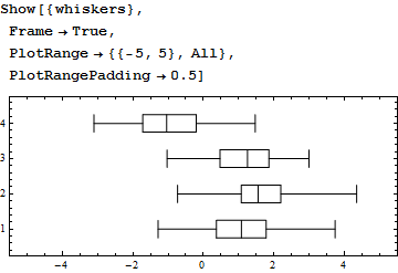
enter image description here

OK, now, I want to show a vertical shaded band between x=-1 and x=1. Conceptually, this is a very simple, commonplace idea, but to do it with Mathematica one must suffer a little...

Note that for the desired modification only two parameters are relevant: the abscissas of the edges of the region of interest. Any $y$-dimension information is completely extraneous to the problem, and can only complicate or sharply reduce the generality of the original figure.

I was not able to find any way to do what I want to do that did not require specifying extraneous, irrelevant parameters. For example:
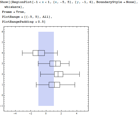
enter image description here

Why did the aspect ratio change? Who knows.

More importantly, notice that for RegionPlot I had to specify the irrelevant range parameters {x, -5, 5} and {y, -1, 6}. These parameters are, in fact, worse than irrelevant: they actually mess up what was there before. For example, now the content-agnostic All spec in the pre-existing PlotRange->{{-5, 5}, All} parameter, and the also content-agnostic PlotRangePadding->0.5 specification, no longer work. I have to replace the first one with a fragile, hard-coded vertical range specification, and fuss with the second one:
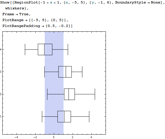
enter image description here

My hope is to find a way to achieve the same effect that is less disruptive, and that it does not force me to specify irrelevant or excessively specific parameters.

$\endgroup$
4
  • 1
    $\begingroup$ Related $\endgroup$
    – Kuba
    Commented Sep 8, 2013 at 14:26
  • $\begingroup$ @Kuba I am impressed that you were able to find this old Q&A to link to the recent one. $\endgroup$
    – Mr.Wizard
    Commented Jun 6, 2017 at 6:48
  • $\begingroup$ @Mr.Wizard The key is to know the answer :) queries like :"is:a Prolog Rectangle" are what I do very often. $\endgroup$
    – Kuba
    Commented Jun 6, 2017 at 6:49
  • $\begingroup$ @Kuba Good advice; thanks. This also gave me a chance to update my answer below which I would not otherwise have thought to do. $\endgroup$
    – Mr.Wizard
    Commented Jun 6, 2017 at 6:56

2 Answers 2

8
$\begingroup$

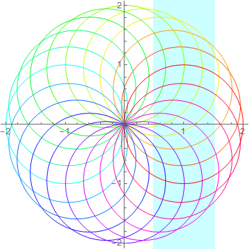
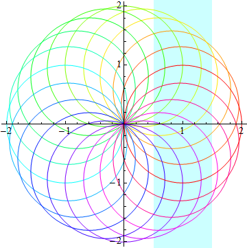
I propose using Prolog and Rectangle:

Graphics[
  Table[{Hue[t/20], Circle[{Cos[2 Pi t/20], Sin[2 Pi t/20]}]}, {t, 20}], 
  Axes -> True,
  Prolog -> {Opacity[0.2, Cyan], Rectangle[{0.5, -1*^4}, {1.5, 1*^4}]}
]

enter image description here

Unfortunately there is no simple way to Combine absolute and relative (scaled) coordinates so I simply used a "large" value for Y limits.


Update

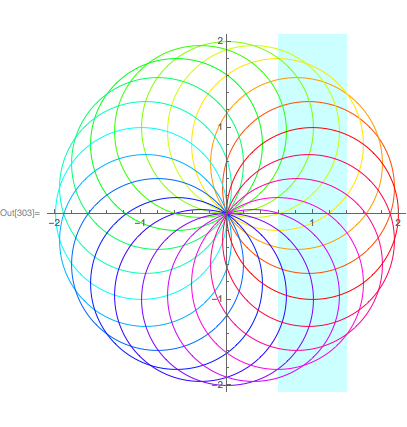
With the introduction of InfiniteLine in Mathematica 10 it is now possible to do this:

Graphics[
  Table[{Hue[t/20], Circle[{Cos[2 Pi t/20], Sin[2 Pi t/20]}]}, {t, 20}], 
  Axes -> True, 
  Prolog -> {Opacity[0.2, Cyan], Thickness[1/4], InfiniteLine[{1, 1}, {0, 1}]}
]

enter image description here

See also:

$\endgroup$
3
  • $\begingroup$ Thank you, that's very instructive. Believe it or not, in this answer, the aspect I find most intriguing (both illuminating and baffling at the same time) is your choice "large" values of $y$, because they strike me as surprisingly modest. In one of my many failed attempts to get this to work, I tried the limits [-big, big] with big = Infinity (naively thinking that Mathematica would surely be hip to this), and when that failed, the more pedestrian big = $MaxMachine, which also failed... $\endgroup$
    – kjo
    Commented Sep 8, 2013 at 15:18
  • 1
    $\begingroup$ ...When I tried such big numbers with your Graphic, the cyan rectangle vanished! In fact, this is the case for any big $> 10^{6.19}$ or so, at least on my hardware, which explains some of my earlier failures (even as it introduces new conundrums, such as why this particular upper limit). Well, at least I've learned that sometimes Mathematica behaves surprisingly parochially in the face of some large numbers! Thanks again! $\endgroup$
    – kjo
    Commented Sep 8, 2013 at 15:18
  • $\begingroup$ @kjo Your right; at first I tried larger values myself but the blue rectangle became invisible when I resized the graphic. I'm afraid Mathematica is ignoring values that are too far out of the specified plot range, or perhaps are too great in magnitude relative to other values. This is worth exploration but I don't have time right now. It would be far better if we could used mixed Scaled coordinates but sadly at this time we cannot. $\endgroup$
    – Mr.Wizard
    Commented Sep 8, 2013 at 15:20
3
$\begingroup$

Another alternative is to use GridLines:

Graphics[
    Table[{Hue[t/20],Circle[{Cos[2 Pi t/20],Sin[2 Pi t/20]}]},{t,20}],
    Axes->True,
    GridLines->{{{1,Directive[Opacity[.2],Cyan,Thickness[1/4]]}},None}
]

yields the same picture as in @MrWizard' s InfiniteLine approach.

Updated to enable specification of left and right abscissa values

Since a pure function GridLines spec receives the plot range, we can use this to construct a Filling that respects a left and right abscissa specification. Here is a pure function that does this:

func[l_,r_] := Function[
    {{(l+r)/2, Directive[Cyan,Opacity[.2],Thickness[(r-l)/(#2-#1)]]}}
]

Draw a rectangle from .6 to 1.4:

Graphics[
    Table[{Hue[t/20],Circle[{Cos[2 Pi t/20],Sin[2 Pi t/20]}]},{t,20}],
    Axes->True,
    GridLines->{func[.6,1.4],None}
]

enter image description here

Addendum

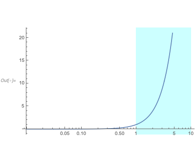
If the plot uses a log scale, you can use the following function instead:

logStrip[l_, r_] := Function[{Print[{##}];
    {
    Exp[(Log@l+Log@r)/2],
    Directive[Cyan, Opacity[.2], Thickness[(Log@r-Log@l)/(#2-#1)]]
    }
}]

Example:

LogLinearPlot[x^2, {x, 0, 10}, GridLines -> {logStrip[1, 10], None}]

enter image description here

$\endgroup$
3
  • $\begingroup$ Is there a general solution to this on a logarithmic axis? In your solution you set the position and thickness in a way that can only be used on linear axes. $\endgroup$
    – DomDoe
    Commented Nov 7, 2019 at 16:46
  • 1
    $\begingroup$ @DomDoe See update. $\endgroup$
    – Carl Woll
    Commented Nov 7, 2019 at 17:19
  • $\begingroup$ Great! Thanks for the quick update! $\endgroup$
    – DomDoe
    Commented Nov 8, 2019 at 9:05

Your Answer

By clicking “Post Your Answer”, you agree to our terms of service and acknowledge you have read our privacy policy.

Not the answer you're looking for? Browse other questions tagged or ask your own question.