11
$\begingroup$

Is this graph in the list among the so-called "standard" structures used in GraphData? However, I have not found yet anything like "Carpet" or "Sponge" in the list of the objects that can be built. Maybe, this graph has a different name?

For me, using GraphData helps to save time for constructing adjacency matrix; therefore, I would rather prefer using this function than drawing the graph...

Thank you very much in advance!

$\endgroup$
1
  • $\begingroup$ Have you seen this? $\endgroup$
    – gpap
    Commented Aug 19, 2013 at 12:47

7 Answers 7

18
$\begingroup$

I don't think there is a carpet graph built-in, but it's hard to be sure that something is not there. Still it's not hard to construct a Graph -- not quite the same thing as drawing it (I wasn't sure what you meant).

There are probably more efficient ways, but adapting Mr.Wizard's carpet function, it is fairly straightforward to make an edge between adjacent 1s in the matrix.

carpet[n_] := (* Mr.Wizard *)
  Nest[ArrayFlatten[{{#, #, #}, {#, 0, #}, {#, #, #}}] &, 1, n];
carpetGraph[n_] := Module[{sa, edges, parts, onesPositions},
  parts = {{1, 0}, {0, 1}};
  sa = SparseArray@carpet[n];
  onesPositions = sa["NonzeroPositions"];
  edges = Flatten[
    With[{m = ArrayPad[sa, 1]}, 
     Function[pos,  pos -> # & /@
        Pick[pos + # & /@ parts, Extract[m, 1 + pos + # & /@ parts], 1]] /@
      onesPositions],
    1];
  Graph[onesPositions, edges, VertexCoordinates -> onesPositions, DirectedEdges -> False]
  ]

g = carpetGraph[4]

Mathematica graphics

You can then compute the adjacency matrix as with any other graph:

(* AdjacencyMatrix[g] // Timing // First *)
(* {0.010865, SparseArray[<12848>, {4096, 4096}]} *)

AdjacencyMatrix[carpetGraph[5]] // Timing
(* {0.878410, SparseArray[<104080>, {32768, 32768}]} *)
$\endgroup$
2
  • $\begingroup$ Michael, I can't run your code because v7 doesn't have Graph but I see that you modified carpet; I'm not sure why. It seems slower than using my original code and converting to a sparse array at the end. I suggest you try this code with my original and then sa = SparseArray @ carpet[n];. Also, you seem to be using sa["NonzeroPositions"] three separate times; why not assign that to an extra Symbol in the Module? $\endgroup$
    – Mr.Wizard
    Commented Aug 20, 2013 at 2:28
  • $\begingroup$ @Mr.Wizard Thanks for the suggestions. I started with the idea of SparseArray and didn't think of applying it at the end. I suppose I could do something about pos + # & /@ parts appearing twice, too. I'm not sure it's worth changing, although the three sa["NonzeroPositions"] seem worth an extra variable. It turns out that the speed is not affected noticeably. (I get roughly equal timings, both faster and slower, up to carpetGraph[6].) My mem. usage would go up 20GB on carpetGraph[5] earlier but not now. Must have been something Mma ate. :) $\endgroup$
    – Michael E2
    Commented Aug 20, 2013 at 3:06
13
$\begingroup$

Here is a "general" Lindenmayer System generator I wrote in the spirit of code-golf. Please beware that the objective of code-golfing is writing the shorter possible program to fulfill an objective, disregarding good practices, robustness, etc. Stay safe and don't use this style in real life.

f[i_, b_, h_, j_, r_, n_] := 
  (a = h; p = j; s = k = {}; t = Flatten;
  (Switch[#,
      6, s = {a, p, s},
      8, {a, p, s} = s,
      _C, k = {k, Black, Line@{p, p += {Cos@a, Sin@a}}},
      _W, k = {k, White, Line@{p, p += {Cos@a, Sin@a}}}];
     If[# < 9, a += I^# b]) & /@ t@Nest[# /. r &, i, n];
  Graphics@t@k)

Where

i : Initial state;
b : rotation angle
h : initial angle
j : initial position
r : production rules
n : iterations

And the production rules for the grammar are:

2 = Turn Left (-);
4 = Turn Right (+);
6 = Push and Turn Left ("[");
8 = Pop and Turn Right ("]");
C[i] = Draw (Any number of symbols)
W[i] = Draw in White (Any number of symbols)
Any other symbol = Do Nothing, just use it in producing next state

So the rules for the carpet are:

f[{C[1]}, Pi/2, 0, {0, 0}, 
  {C@1 -> {C@1, 4, C@1, 2, C@1, 2, C@1, 2, W@3, 4, C@1, 4, C@1, 4, C@1, 2, C@1}, 
   W@3 -> {W@3, W@3, W@3}}, 5]

Mathematica graphics

Other usage examples (sorry, couldn't resist)

Examples:

f[{C@1, X}, Pi/2, 0, {0, 0}, {X -> {X, 4, Y, C@1}, Y -> {C@1, X, 2, Y}}, 10]
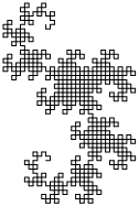
Mathematica graphics

f[{C@1}, Pi/2, 0, {0,0}, {C@1->{C@1, 2, C@1, 4, C@1, 4, C@1, 2, C@1}}, 6]
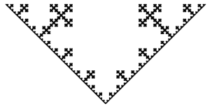
Mathematica graphics

f[{C@1}, Pi/4, Pi/2, {0, 0}, {C@2 -> {C@2, C@2}, C@1 -> {C@2, 6, C@1, 8, C@1}}, 10]
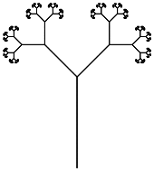
Mathematica graphics

f[{C[1]}, Pi/3, 0, {0, 0}, 
  {C@1 -> {C@2, 4, C@1, 4, C@2}, C@2 -> {C@1, 2, C@2, 2, C@1}}, 10]
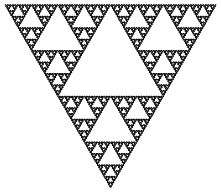
Mathematica graphics

f[{X},5/36 Pi, Pi/3, {0,0},
 {X->{C@1, 4, 6, 6, X, 8, 2, X, 8, 2, C@1, 6, 2, C@1, X, 8, 4, X}, 
 C@1->{C@1, C@1}}, 6]
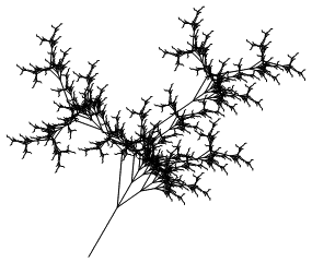
Mathematica graphics

Edit

Since you wanted a Graph ... here it is:

f[i_, b_, h_, j_, r_, n_] := (a = h; p = j; s = k = {}; g =.;
   t = Flatten;
   (Switch[#,
       6, s = {a, p, s},
       8, {a, p, s} = s,
       _C, AppendTo[k, {p, (p += {Cos@a, Sin@a})}],
       _W, p += {Cos@a, Sin@a}];
      If[# < 9, a += I^# b]) & /@ t@Nest[# /. r &, i, n];);
f[{C[1]}, Pi/2, 0, {0, 0}, 
   {C@1 -> {C@1, 4, C@1, 2, C@1, 2, C@1, 2, W@3, 4, C@1, 4, C@1, 4, C@1, 2, C@1}, 
    W@3 -> {W@3, W@3, W@3}}, 2];

g = Graph[Rule @@@ k];
(PropertyValue[{g, #}, VertexCoordinates] = #) & /@ VertexList@g;
g
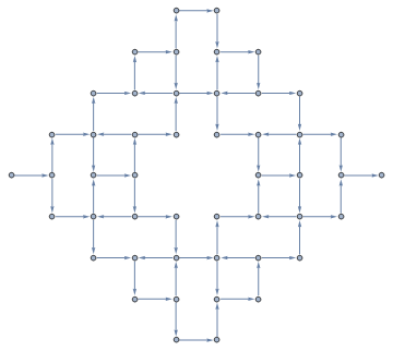
Mathematica graphics

If you let Mathematica to place the Vertices automagically, you also get nice pictures

Mathematica graphics

$\endgroup$
6
  • 1
    $\begingroup$ That sure looks nice, but since this isn't Code Golf you should probably localize your variables. Also, how long is this supposed to take to render? I tried the first example before starting to write this comment, and it's still running. (Okay, it just finished. +1) $\endgroup$
    – Mr.Wizard
    Commented Aug 21, 2013 at 0:22
  • $\begingroup$ Well I just lifted my vote. This is undoubtedly cool but I don't think it answers the question, which I think is about Graph data as Michael's answer produces. $\endgroup$
    – Mr.Wizard
    Commented Aug 21, 2013 at 0:25
  • $\begingroup$ @Mr.Wizard Now it does Graphs :) $\endgroup$ Commented Aug 21, 2013 at 0:59
  • $\begingroup$ Noted and vote restored. Please consider adding Module still; it's just bad practice not to, outside of Code Golf. $\endgroup$
    – Mr.Wizard
    Commented Aug 21, 2013 at 1:00
  • 4
    $\begingroup$ "I cannot agree with those who rank modesty among the virtues." Sherlock Holmes :) $\endgroup$
    – cormullion
    Commented Aug 21, 2013 at 14:23
7
$\begingroup$

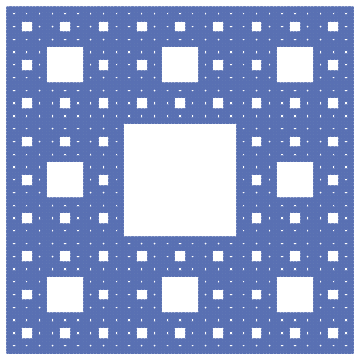
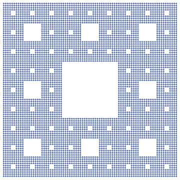
As of version 11, this is built in:

GraphData["SierpinskiCarpet"]
(* {{"Cycle", 8}, {"SierpinskiCarpet", 2}, {"SierpinskiCarpet", 3}, {"SierpinskiCarpet", 4}} *)

GraphData /@ %

Mathematica graphics


The latest version of IGraph/M incorporates Henrik Schumacher's mesh/graph conversion functions. This way we can easily obtain the face-adjacency graph of a MengerMesh, and add the appropriate vertex coordinates.

Needs["IGraphM`"]

With[{mesh = MengerMesh[4]},
 IGMeshCellAdjacencyGraph[mesh, 2,
  VertexCoordinates -> PropertyValue[{mesh, {2, All}}, MeshCellCentroid]
 ]
]

Mathematica graphics

How about a 3D one?

With[{mesh = MengerMesh[2, 3]},
 IGMeshCellAdjacencyGraph[mesh, 3,
  VertexCoordinates -> PropertyValue[{mesh, {3, All}}, MeshCellCentroid]
 ]
]

Mathematica graphics

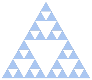
What if we want a Sierpinski graph? The mesh looks like this:

mesh = SierpinskiMesh[3]

Mathematica graphics

This time each face (shaded triangle) will correspond to a graph node, and two triangles are connected if they share a vertex. We construct the face-vertex incidence matrix bm. To obtain our graph's adjacency matrix, we need those elements of bm.Transpose[bm] which are 1. We enlist the help of the BoolEval package for this.

bm = IGMeshCellAdjacencyMatrix[mesh, 2 (* face, i.e. 2D *), 0 (* vertex, i.e. 0D *)];

Needs["BoolEval`"]

AdjacencyGraph[
 BoolEval[bm.Transpose[bm] == 1],
 VertexCoordinates -> PropertyValue[{mesh, {2, All}}, MeshCellCentroid]
]

Mathematica graphics

$\endgroup$
3
  • $\begingroup$ Since we are in 11.1,why not use MengerMesh? $\endgroup$
    – yode
    Commented May 5, 2017 at 17:12
  • $\begingroup$ @yode See my comment on Chip's answer. $\endgroup$
    – Szabolcs
    Commented May 5, 2017 at 19:24
  • $\begingroup$ @yode I added a solution using MengerMesh now. $\endgroup$
    – Szabolcs
    Commented Dec 4, 2017 at 21:42
3
$\begingroup$

If we are in 11.1, we can use in-built function MengerMesh.Well,I always faced a problem about grid layout.Whatever it is simple enough to plot Sierpinski

AdjacencyGraph[Graphics`Region`ToMeshObject[MengerMesh[4]]["AdjacencyMatrix"]]

Mathematica graphics


Update

I have found a properties of mesh object "VertexCoordinateRules".It is can serve a good grid layout for this case.

mesh = Graphics`Region`ToMeshObject[MengerMesh[4]];
g = AdjacencyGraph[mesh["AdjacencyMatrix"]];
Graph[g, VertexCoordinates -> mesh["VertexCoordinateRules"]]

Mathematica graphics

Of course we can change the MengerMesh into SierpinskiMesh or CantorMesh,then we can get

Mathematica graphics

$\endgroup$
2
$\begingroup$

The mesh-related functionality in current versions allows for relatively compact code for generating the graph version of the Sierpinski carpet. The following solution is more or less similar to this previous answer:

pos = DeleteCases[Tuples[2 {-1, 0, 1}/3, {2}], {0, 0}];

With[{n = 5},
     sqrs = Flatten[Nest[# /. Rectangle[p1_, p2_] :>
                         Map[Rectangle[p1/3 - #, p2/3 - #] &, pos] &,
                         Rectangle[-{1, 1}, {1, 1}], n]];
     pts = Flatten[Tuples[Transpose[{##}]][[{1, 2, 4, 3}]] & @@@ sqrs, 1];
     mr = MeshRegion[pts, Polygon[Partition[Range[Length[pts]], 4]]];
     Graph[Range[MeshCellCount[mr, 0]], UndirectedEdge @@@ (First /@ MeshCells[mr, 1]), 
           EdgeShapeFunction -> "Line", VertexCoordinates -> MeshCoordinates[mr],
           VertexSize -> Small]]

Sierpinski carpet graph


The code for the Menger sponge's graph version is similarly compact:

pos = Select[Tuples[2 {-1, 0, 1}/3, {3}], (Count[#, 0] < 2) &];

With[{n = 3},
     cubs = Flatten[Nest[# /. Cuboid[p1_, p2_] :>
                         Map[Cuboid[p1/3 - #, p2/3 - #] &, pos] &, 
                         Cuboid[-{1, 1, 1}, {1, 1, 1}], n]];
     pts = Flatten[Tuples[Transpose[{##}]][[{1, 5, 7, 3, 2, 6, 8, 4}]] & @@@ cubs, 1];
     mr = BoundaryMesh[MeshRegion[pts, Hexahedron /@ Partition[Range[Length[pts]], 8]]];
     Graph3D[Range[MeshCellCount[mr, 0]], UndirectedEdge @@@ (First /@ MeshCells[mr, 1]), 
             EdgeShapeFunction -> "Line", VertexCoordinates -> MeshCoordinates[mr],
             VertexSize -> Small]]

Menger sponge graph

$\endgroup$
2
$\begingroup$

Since V 11.1 we have MengerMesh

MengerMesh[3]

enter image description here

MengerMesh[3, 3]

enter image description here

Other iterated maps include SierpinskiMesh, CantorMesh and ArrayMesh. A full listing is here:

Iterated Maps & Fractals

Just for fun:

k = 12;

r = #2 /. {x__Real} :> .1 {{7, -#}, {#, 7}} . {x} + y &;

f[n_] := {f @ 1 = N @ Polygon @ {y = {0, .7^k}, 0 y, x = {.002, 0}, x + y}, r[-4, p = f[n - 1]], 4~r~p}

Graphics @ f @ k

enter image description here

Source: Create a fractal tree

$\endgroup$
1
$\begingroup$

Version 12.1 now has the function MeshConnectivityGraph[] which can be used on MengerMesh[]:

MeshConnectivityGraph[MengerMesh[4, 2], PlotTheme -> "LargeNetworkDefault"]

Sierpinski carpet graph

MeshConnectivityGraph[MengerMesh[2, 3], PlotTheme -> "LargeNetworkDefault"]

Menger sponge graph

$\endgroup$

Your Answer

By clicking “Post Your Answer”, you agree to our terms of service and acknowledge you have read our privacy policy.

Not the answer you're looking for? Browse other questions tagged or ask your own question.