Using NDSolve to solve the PDEs and their reduced ODEs yields inconsistent results

Question

I am working with a system of coupled PDEs: \begin{align} \partial_tP_x(t,x)&=(\omega_0+\gamma gx)P_y(t,x)-P_x(t,x)/T_2+D\partial_x^2P_x(t,x)\\ \partial_tP_y(t,x)&=-(\omega_0+\gamma gx)P_x(t,x)-P_y(t,x)/T_2+D\partial_x^2P_y(t,x) \end{align} subject to the boundary condition $\partial_xP_{x,y}(t,x)|_{x=\pm L/2}=0$.

Before solving the above PDEs, I did a test the system by setting $g=0,D=0,T_2\rightarrow\infty$, which reduces the PDEs to the following ODEs:

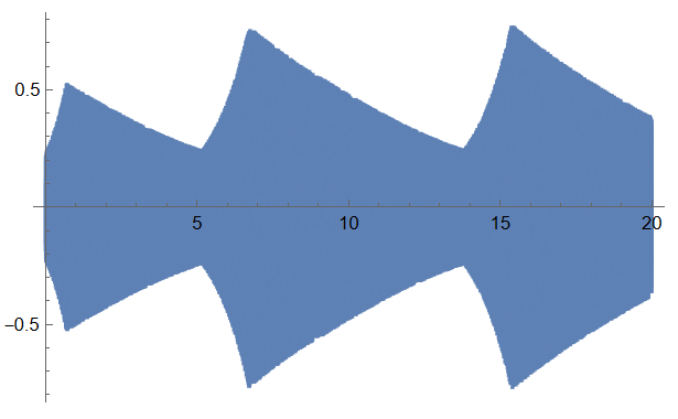
\begin{align} \partial_tP_x(t,x)&=\omega_0P_y(t,x)\\ \partial_tP_y(t,x)&=-\omega_0P_x(t,x) \end{align} which has the exact solution $P_x(t)\sim\cos(\omega_0t+\phi)$. However, when I keep the varialbe x, NDsolve gives the unexpected results. Here’s the code:

gamma = -2*Pi*1.18*10^7;
T20 = 1/0.306;
T10 = 400;
P0 = 0.5;
omega0 = 2*Pi*257.45;


L = 0.8;
diffusion = 0  0.211;

datag = Table[o, {o, 10, 300, 10}] 10^-9;
g = 0  300  10^-9;
omega[z_] := omega0 + (gamma*g*z);
pde = {D[Px[t, x], t] == 
    diffusion  D[Px[t, x], x, x] + Py[t, x] omega[x](*-Px[t,x]/T20*), 
   D[Py[t, x], t] == 
    diffusion  D[Py[t, x], x, x] - Px[t, x] omega[x](*-Py[t,x]/T20*)};

pdebc = {(*(D[Px[t,x],x]/.{x\[Rule]L/2})== 0,(D[Px[t,x],
   x]/.{x\[Rule]-L/2})== 0,(D[Py[t,x],x]/.{x\[Rule]L/2})== 0,(D[Py[t,
   x],x]/.{x\[Rule]-L/2})== 0,*)Px[0, x] == Sin[Pi/15], 
   Py[0, x] == 0};


solpde = NDSolve[{pde, pdebc}, {Px, Py}, {x, -L/2, L/2}, {t, 0, 20}];
Plot[Evaluate[Px[t, 0] /. First[solpde]], {t, 0, 20}(*,{x,-L/2,L/2}*),
  PlotRange -> All, PlotPoints -> 200]

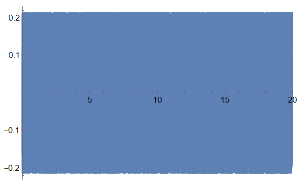
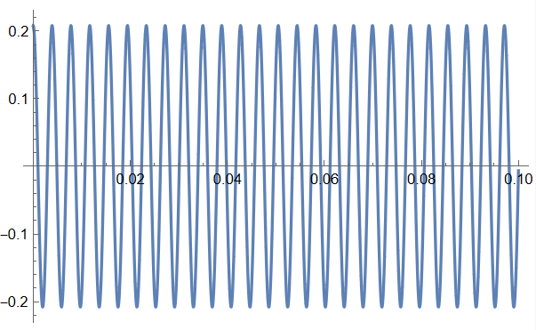
Obviously, it's inconsistent with the exact solution. On the other hand, solving the system of ODEs by ignoring x gives the correct behavior

ode = {D[Px[t], t] == Py[t] omega[x], 
   D[Py[t], t] == -Px[t] omega[x]};
odebc = {Px[0] == Sin[Pi/15], Py[0] == 0};
solode = NDSolve[{ode, odebc}, {Px, Py}, {t, 0, 20}];
Plot[Evaluate[Px[t] /. First[solode]], {t, 0, 20}(*,{x,-L/2,L/2}*), 
 PlotRange -> All, PlotPoints -> 200]

with details

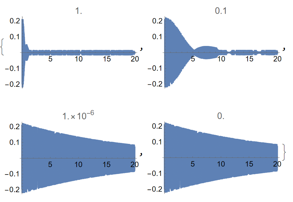
So, what is the issue here? Can I trust NDSolve for solving PDEs in this situation?

Answer 1

Here we have a typical artificial viscosity effect. To make this effect more visible, we will apply FEM to solve the problem as follows.

Needs["NDSolve`FEM`"];
gamma = -2*Pi*1.18*10^7;
T20 = 1/0.306;
T10 = 400;
P0 = 0.5;
omega0 = 2*Pi*257.45;
L = 0.8;
diffusion = 0.211; reg = ImplicitRegion[-L/2 <= x <= L/2, {x}]; mesh =
  ToElementMesh[reg]


datag = Table[o, {o, 10, 300, 10}]  10^-9;
g = 300   10^-9;
omega[z_] := omega0 + k (gamma*g*z);
pde = {D[Px[t, x], t] == 
    k  diffusion   D[Px[t, x], x, x] + Py[t, x]  omega[x], 
   D[Py[t, x], t] == 
    k  diffusion   D[Py[t, x], x, x] - Px[t, x]  omega[x]};

pdebc = {Px[0, x] == Sin[Pi/15], Py[0, x] == 0};
sol[k0_] := 
  NDSolve[{pde, pdebc} /. k -> k0, {Px, Py}, {t, 0, 20}, 
   Element[{x}, mesh]];

Please, note, that the zero Neumann boundary conditions are automatically applied to both ends of reg. Using parameter k we can visualize the artificial viscosity effect as

solk = sol[#] & /@ {1, .1, 10^-6, 0};

Table[Plot[Evaluate[Px[t, 0] /. solk[[i]][[1]]], {t, 0, 20}, 
  PlotRange -> All, PlotLabel -> N@{1, .1, 10^-6, 0}[[i]]], {i, 4}] 

As we can see from the figures above, the vibration energy is lost due to artificial viscosity. To avoid these losses, it is necessary to build a special algorithm.