6
$\begingroup$

Suppose some data with no regular pattern is given, so common patterns of functions all fail to fit it. Then how can one find the best fitting curve? I believe there will be some data for which we can not find any regular pattern. One can try with the following data (luckily, we know that this sequence has a limit):

  {{1, 0.08888888888888872},{2, 0.13842641081508972},{3, 0.17153280014540232},
   {4, 0.19586894934728782},{5, 0.21482500502852542},{6, 0.23017213935351592},
   {7, 0.24294479920054762},{8, 0.25379708095478332},{9, 0.26316771779066082},
   {10, 0.27136463872018062},{11, 0.27861184976714762},{12, 0.28507709754351612},
   {13, 0.29088903838678592},{14, 0.29614834727916052},{15, 0.30093516063430942},
   {16, 0.30531421254734282},{17, 0.30933847047870212},{18, 0.31305176609215322},
   {19, 0.3164907360488469}}

Any help or suggestion will be appreciated!

$\endgroup$
1
  • $\begingroup$ This reply of mine fits inerpolation functions to data. No equation is used. $\endgroup$
    – Hugh
    Commented Jul 17, 2015 at 20:03

6 Answers 6

8
$\begingroup$

May be something here of use: https://mathematica.stackexchange.com/a/14232/363

data=
{{1, 0.08888888888888872},{2, 0.13842641081508972},{3, 0.17153280014540232},
 {4, 0.19586894934728782},{5, 0.21482500502852542},{6, 0.23017213935351592},
 {7, 0.24294479920054762},{8, 0.25379708095478332},{9, 0.26316771779066082},
 {10, 0.27136463872018062},{11, 0.27861184976714762},{12, 0.28507709754351612},
 {13, 0.29088903838678592},{14, 0.29614834727916052},{15, 0.30093516063430942},
 {16, 0.30531421254734282},{17, 0.30933847047870212},{18, 0.31305176609215322},
 {19, 0.3164907360488469}};

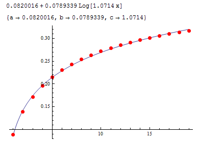
nlm = NonlinearModelFit[data, {a + b Log[c x], c > 0}, {a, b, c}, x];
Print@Normal@nlm;
Print@FindFit[data, {a + b Log[c x], c > 0}, {a, b, c}, x];
Show[Plot[nlm[x], {x, 1, Length@data}, PlotRange -> All],
 ListPlot[data, PlotStyle -> Directive[Red, PointSize[0.02]]]]

enter image description here

See also, http://reference.wolfram.com/mathematica/tutorial/CurveFitting.html - particularly the section: 'Searching for general fits to data'.

$\endgroup$
4
  • $\begingroup$ Thanks very much! As the example in the question, I can give more data and the sequence has a limit. But in more general case waht if we can not find a common pattern of function to fit the data very well? $\endgroup$ Commented Aug 15, 2013 at 10:12
  • $\begingroup$ I've added a link to the curve fitting tutorial. There are only a few general cases to try before one may need to resort to a polynomial fit. $\endgroup$ Commented Aug 15, 2013 at 10:19
  • 1
    $\begingroup$ Thanks a lot! As the example in the question, I have try some possible cases. Since the sequence will converge, a polynomial fit will not help after all. $\endgroup$ Commented Aug 15, 2013 at 10:41
  • $\begingroup$ Just for the record: When the sequence will converge, a logarithmic model is not suitable. $\endgroup$
    – DPF
    Commented Oct 17, 2016 at 20:41
6
$\begingroup$

In version 10.2 there is a new experimental function which might be what you are looking for: FindFormula.

I suspect that a genetic programming algorithm (symbolic regression) is behind this new feature.

See also my question here: What is behind experimental function: FindFormula?

$\endgroup$
1
  • 3
    $\begingroup$ Sadly, this dataset is too small for FindFormula to produce sensible results. Some of its' fits are pretty nice, but at least in this case it also produces plenty of fits which are total garbage from an intuitive standpoint. I believe FindFormula needs datasets to be at least a magnitude larger not to suffer from crazy over-fitting. It's also notable that FindFormula depends on randomness on its' search; it may return different results on every invocation. $\endgroup$
    – kirma
    Commented Jul 18, 2015 at 6:47
4
$\begingroup$

Functions are like vectors. Actually you can define a vector space over functions. We can describe any vector in terms of 3 independent vector which may not be orthogonal to each other. Similarly, you can fit a function in terms of other linearly independent functions. The easiest case is fitting to a polynomial of order n. Depending on how well your data can be fit you can set n. Another example is fitting to a series of Sine and Cose functions(Discrete Fourier transform). One other example is fitting to Gaussian functions with different mean and standard deviation.

data = {{1, 0.08888888888888872}, {2, 0.13842641081508972}, {3, 
0.17153280014540232}, {4, 0.19586894934728782}, {5, 
0.21482500502852542}, {6, 0.23017213935351592}, {7, 
0.24294479920054762}, {8, 0.25379708095478332}, {9, 
0.26316771779066082}, {10, 0.27136463872018062}, {11, 
0.27861184976714762}, {12, 0.28507709754351612}, {13, 
0.29088903838678592}, {14, 0.29614834727916052}, {15, 
0.30093516063430942}, {16, 0.30531421254734282}, {17, 
0.30933847047870212}, {18, 0.31305176609215322}, {19, 
0.3164907360488469}};

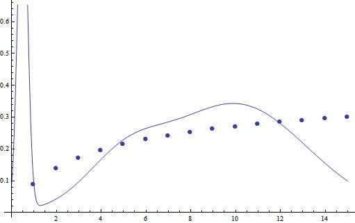
Fit to Cos functions:

model2 = Sum[Subscript[a, n]*Cos[(2*Pi)/T*n*x], {n, 0, 20}];
sol = FindFit[data , {model2, T > 100},  Flatten[{Table[{Subscript[a, i]}, {i, 0, 20}], T}], x]

enter image description here

Fit to polynomial:

model1 = Sum[Subscript[a, i]*x^i, {i, 0, 5}];
sol = FindFit[data , {model1},  Flatten[{Table[{Subscript[a, i]}, {i, 0, 5}]}], x]

enter image description here

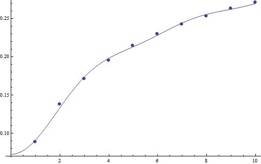
Fit to Gaussian functions:

enter image description here

Here I took only 3 Gaussian function, for better fit either you need more Gaussian functions or a better initial guess and constraints.

$\endgroup$
1
$\begingroup$

How about a mixture of smoothing and curve fitting? This is based on a previous post of mine here. We use a best interpolation function. Here is your data.

data = {{1, 0.08888888888888872}, {2, 0.13842641081508972}, {3, 
    0.17153280014540232}, {4, 0.19586894934728782}, {5, 
    0.21482500502852542}, {6, 0.23017213935351592}, {7, 
    0.24294479920054762}, {8, 0.25379708095478332}, {9, 
    0.26316771779066082}, {10, 0.27136463872018062}, {11, 
    0.27861184976714762}, {12, 0.28507709754351612}, {13, 
    0.29088903838678592}, {14, 0.29614834727916052}, {15, 
    0.30093516063430942}, {16, 0.30531421254734282}, {17, 
    0.30933847047870212}, {18, 0.31305176609215322}, {19, 
    0.3164907360488469}};

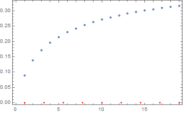
Now define a number of control points. This number must be less than the number of your data points. The more control points the closer the fit to your data but the less smooth the fitted curve.

nOfControlPoints = 9;
controlPoints = 
  Subdivide[#1, #2, nOfControlPoints - 1] & @@ MinMax[data[[;; , 1]]];
ListPlot[data, Epilog -> {Red, Point[{#, 0}] & /@ controlPoints}, 
 Frame -> True, Axes -> False]

Mathematica graphics

Now fit the model.

   model[y : {__Real}] := Interpolation[Transpose[{controlPoints, y}]];
    nlm = NonlinearModelFit[data, model[Array[y, nOfControlPoints]][x], 
       Array[y, nOfControlPoints], x];

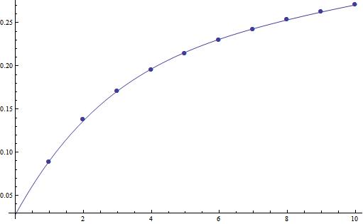
Plot the data and the fitted curve.

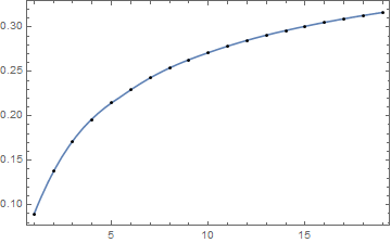
   Plot[nlm["Function"][x], {x, data[[1, 1]], data[[-1, 1]]}, 
     Epilog -> {Point[data]}, Frame -> True]

Mathematica graphics

The advantage of this method is that it avoids the use of polynomials which always give a poor fit when the order is high. Very large data sets can be fitted with a smooth curve using this method. Hope this helps.

$\endgroup$
6
  • $\begingroup$ Interesting approach, but I find the term "model" kind of misleading, as it is just a smoothing and no "real" model, motivated by physics or other processes. $\endgroup$
    – DPF
    Commented Oct 17, 2016 at 18:04
  • $\begingroup$ @DPF I agree with your comment. If you have some physics then you should try and get that into the model. However, if you don't know why the function behaves as it does then at least you can do some maths with this model. If you blindly fit polynomials that usually goes wrong. $\endgroup$
    – Hugh
    Commented Oct 17, 2016 at 18:28
  • $\begingroup$ For this case are very powerful interpolation tools available. $\endgroup$
    – DPF
    Commented Oct 17, 2016 at 19:05
  • $\begingroup$ @DPF Sorry is that a question or a statement? $\endgroup$
    – Hugh
    Commented Oct 17, 2016 at 19:49
  • $\begingroup$ My comment has no question mark, that makes it a statement ;). I recommend not to use the terms "fit" and "model" for the process of interpolation. $\endgroup$
    – DPF
    Commented Oct 17, 2016 at 20:43
1
$\begingroup$

Since it was mentioned that the sequence is expected to have a limit then the log function proposed as an answer wouldn't work since it would go to infinity. Possibly an equation of the following form would be better suited since it does have a limit.

$a\, -\frac{b}{\sqrt{\text{X}+c}}$

Using NonlinearModelFit with this form will as shown below will lead to the equation

NonlinearModelFit[data1, a - b/Sqrt[c + x], {a, b, c}, x]

$0.455437\, -\frac{0.638033}{\sqrt{x+2.03654}}$

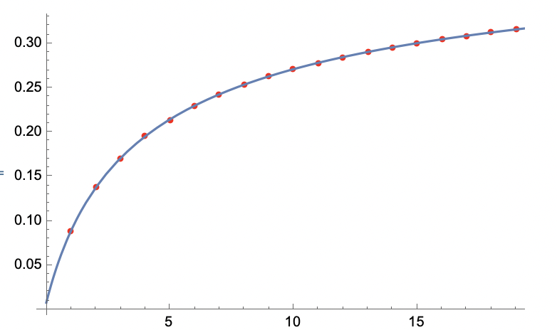
The fit is shown below. We can see that it fits the data very well. As well, it will approach the limit of 0.455437...

Show[ListPlot[data1,PlotStyle->Red],Plot[0.4554374226267565` -0.6380326609461318`/Sqrt[2.0365359603988993` +x],{x,0,20}]]

enter image description here

$\endgroup$
1
  • $\begingroup$ @MichaelE2 Updated the answer to better explain the use of Mathematica and also optimized the value for "c" instead of approximating it with an integer to give the best possible fit. $\endgroup$
    – Nate
    Commented Jun 24, 2022 at 17:43
0
$\begingroup$

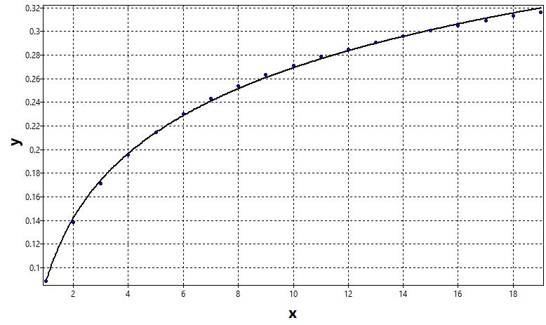
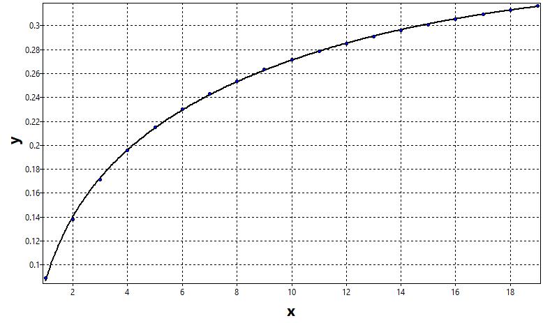
Is that what you mean? Model 1: y= a0 + a1*ln(x), a0 = 0.0874214, a1 = 0.0789488

Model1

Model 2: y= a0 + a1*x^(1/7) + a2*(ln(x))^5 a0= -4.04E-01, a1 = 0.4928045, a2 = -1.36E-04

Model2

Calculated using ndCurveMaster

$\endgroup$
1
  • 1
    $\begingroup$ Did you use Mathematica to carry out these fitting calculations? $\endgroup$
    – MarcoB
    Commented May 22, 2017 at 13:17

Your Answer

By clicking “Post Your Answer”, you agree to our terms of service and acknowledge you have read our privacy policy.

Not the answer you're looking for? Browse other questions tagged or ask your own question.