20
$\begingroup$

Bridget Riley

Bridget Riley (born 1931 in London) is an English painter known for her op art paintings. Alongside Victor Vasarely and Vera Molnár, she is one of the best-known representatives of this art movement.

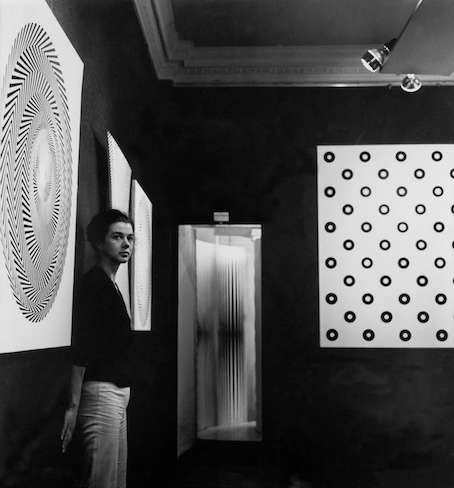
enter image description here

Bridget Riley at Gallery One, London, 1963

Riley studied art at Goldsmiths' College (1949–52), and later at the Royal College of Art (1952–55). During the early 1960s Riley began to paint the black and white works for which she first became known. They present a great variety of geometric forms that produce sensations of movement or colour. Riley began investigating colour in 1967, the year in which she produced her first stripe painting.

enter image description here

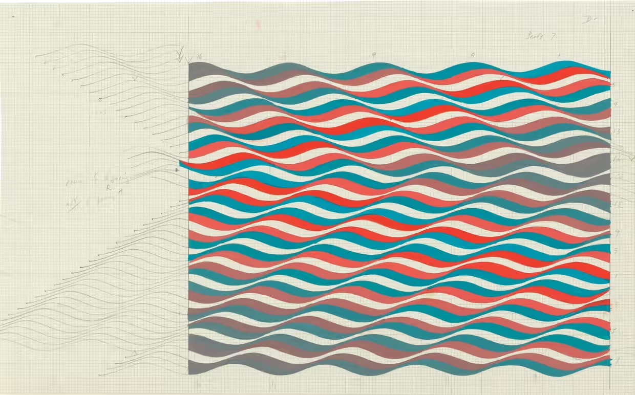
Bridget Riley, preparatory drawing, 1968

As seen above Riley meticulously plans her compositions with preparatory drawings and collage techniques. Her assistants then paint the final canvases with great precision under her instruction.

Bridget Riley's works are featured in major international museums, including MoMA, NewYork and Tate Modern, London.

Movement in Squares

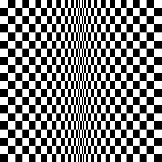
This seminal painting from 1961 marks Riley’s first major breakthrough into abstraction. Using the simple form of the square, she achieved perceptual effects of motion and space that paved the way for her subsequent black-and-white paintings.

enter image description here

Bridget Riley, Movement in Squares (left) and my reproduction (right)

Despite the seemingly simple pattern I couldn't find an algorithmic solution and had to "manually" insert the rectangle coordinates:

squares[{c_, d_}] :=
 With[{r = Rectangle},
  {c, r[{0.0, i}, {1.0, i + 1}], d, r[{1.0, i}, {2.0, i + 1}],
   c, r[{2.0, i}, {2.9, i + 1}], d, r[{2.9, i}, {3.8, i + 1}],
   c, r[{3.8, i}, {4.6, i + 1}], d, r[{4.6, i}, {5.4, i + 1}],
   c, r[{5.4, i}, {6.1, i + 1}], d, r[{6.1, i}, {6.8, i + 1}],
   c, r[{6.8, i}, {7.4, i + 1}], d, r[{7.4, i}, {8.0, i + 1}],
   c, r[{8.0, i}, {8.5, i + 1}], d, r[{8.5, i}, {9.0, i + 1}],
   c, r[{9.0, i}, {9.4, i + 1}], d, r[{9.4, i}, {9.8, i + 1}],
   c, r[{9.8, i}, {10.1, i + 1}], d, r[{10.1, i}, {10.4, i + 1}],
   c, r[{10.4, i}, {10.6, i + 1}], d, r[{10.6, i}, {10.8, i + 1}],
   c, r[{10.8, i}, {10.9, i + 1}], d, r[{10.9, i}, {11.0, i + 1}],
   c, r[{11.0, i}, {11.1, i + 1}], d, r[{11.1, i}, {11.2, i + 1}],
   c, r[{11.2, i}, {11.3, i + 1}], d, r[{11.3, i}, {11.5, i + 1}],
   c, r[{11.5, i}, {11.8, i + 1}], d, r[{11.8, i}, {12.1, i + 1}],
   c, r[{12.1, i}, {12.5, i + 1}], d, r[{12.5, i}, {12.9, i + 1}],
   c, r[{12.9, i}, {13.4, i + 1}], d, r[{13.4, i}, {13.9, i + 1}],
   c, r[{13.9, i}, {14.5, i + 1}], d, r[{14.5, i}, {15.1, i + 1}],
   c, r[{15.1, i}, {15.8, i + 1}], d, r[{15.8, i}, {16.5, i + 1}]}]

bw = squares[{Black, GrayLevel[1]}];
wb = squares[{GrayLevel[1], Black}];

Graphics[Table[{bw, wb}[[Mod[i, 2] + 1]], {i, 1, 15}], AspectRatio -> 1]

Result like shown above

Movement in Circles

enter image description here

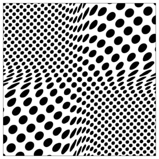
Bridget Riley, Pause, 1964

Question

I want to find an elegant, algorithmic way to reproduce "Movement in Squares". Since my ultimate goal is to replicate "Pause" (shown above), I would be particularly grateful for solutions that also address the latter.

$\endgroup$
3
  • 5
    $\begingroup$ I like your posts very much and I think the art-math connection is an excellent way to demonstrate the MA capabilities. They would be even better if follow some logical rules on what constitute a solution. For instance, the accepted answer (1st part) does not even answer your question(s). And the 2nd part (to my humble opinion) is not better than numerous other answers. I think, these enthusiastic people working hard on solving your problems deserve at least an explanation on what motivated your choice of winner. This is certainly not the time order, nor the completeness or generality order. $\endgroup$
    – yarchik
    Commented Apr 23 at 11:49
  • 2
    $\begingroup$ Thanks for your feedback, yarchik. I agree that other answers (all of them are great and deserve acceptance) more closely stick to the question. My explanation: I was somehow overwhelmed by the pure beauty of azerbajdjan's first answer (the colour waves). I had worked for hours without too much success on these sinusoids (see my comment under his answer), and didn't even dare to pose it as a question because it seemed so complicated. In the future I will try to better match question and acceptance. Promised. And last but not least: Thanks to everybody for the beautiful answers. $\endgroup$
    – eldo
    Commented Apr 23 at 13:47
  • $\begingroup$ For the first picture, it seems like the propagation of the wave, maybe we can consider the wave equation to get the general drawing method, but upto now it still difficult for me, so I concentrate at the last picture :) $\endgroup$
    – cvgmt
    Commented Apr 23 at 14:22

5 Answers 5

21
$\begingroup$

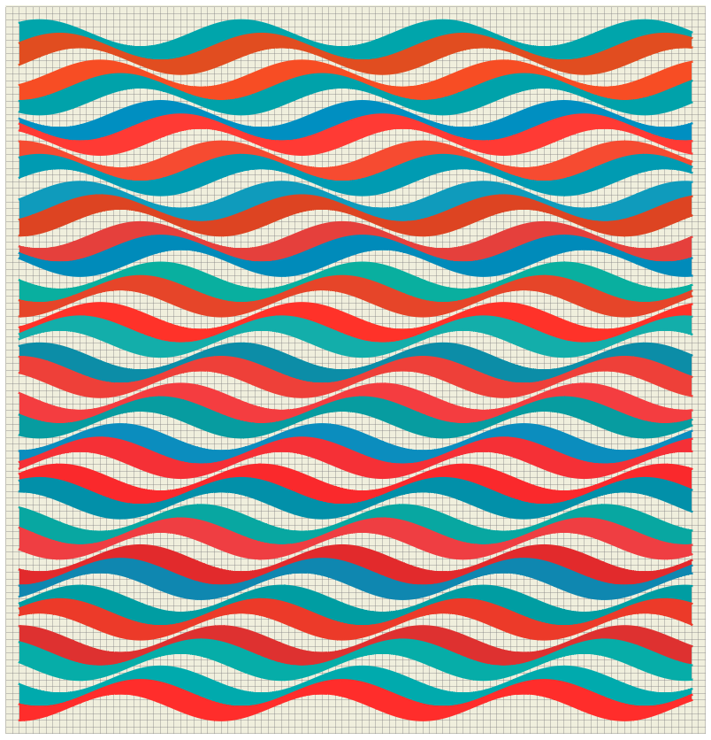
Since I like the color image more than the black-and-white...

c1 := RGBColor[({0, 155, 175} + RandomInteger[{-20, 20}, 3])/255]
c2 := RGBColor[({238, 60, 46} + RandomInteger[{-20, 20}, 3])/255]
color := {c1, c2, None, c2, c1, None}
fil = MapIndexed[#[[1]] -> {{#[[2]]}, color[[Mod[First@#2, 6, 1]]]} &,
    Partition[Range[51], 2, 1]];
style = Flatten[
   Append[#, #[[2]]] & /@ 
    Partition[DeleteCases[fil[[All, 2, 2]], None], 2]];

Plot[Evaluate@
  Join[Table[
    1/5 (1 + n - Cos[(n Pi)/5 + (2 Pi x)/3]), {n, 14, -3, -1}], 
   Table[1/5 (-5 - n - Cos[(n Pi)/5 + (2 Pi x)/3]), {n, -2, 30}]], {x,
   0, 10}, Filling -> fil, AspectRatio -> Automatic, 
 GridLines -> {Range[-2, 12, 0.1], Range[-8, 4, 0.1]}, 
 PlotStyle -> style, Axes -> False, 
 PlotRange -> {{-0.2, 10.21}, {-7.41, 3.4}}, ImagePadding -> 0.1, 
 Background -> RGBColor[{240, 239, 221}/255]]

enter image description here

"1:eJytU11v0zAU3Qu/gD9QNGlq1evWdpKt+2i1rqzTEENVy5vrBy8xJcKzoySDjCj/\
HdupYIixVYIX+9q+9/j43OM3t2a5ev1qby8mJ+\
Pl1cXMKJOzbo2BRBGQo6jpL4VOzN21LuVG5qxGFAPFDQS8N6RRxNeY0Jj+\
VkyDERxiCA93K3ZVJ+M6JhBT+\
GC0dLNdubBxGZ9SNb4R2bVOZCUTts8Y4RxN6tpGlPMGPARjNyZh8zQvyvN9Codgk3hzAAu\
Rl2mZGs0smY1kEeFA3eGpwy7KByXHcyXKUmo2zTKp7Q3QIvOD4fmv8rdSyVLORCELZikxN\
lXKItk8T5W76HR9Mg+mgUPOyHihTMkuvwp1L0p5/\
s6kmn0Ut0oyMow6XdLXaGYK1tWdRdobRv0utUGn6g2tPFBrICGgABBpODwqQxF6oQ5RCHB\
jadUV2EYGg+MG5qlSqd6giWUO0yKTcbkU9lloMr0vzZ0NY7jK0+\
R9qmVhtW21skgkHBDAAyvadmsEoV834J63cvqhiZcRppWrnQtVSH/\
oK1yjEB60SA3U6GgQQjAImwau78RGLkSSeGYWFC5E/\
GWTm3udoMlPR9U0tLYJjoFS0njf8FbmjP5d4pnRie+bUJdVlsuicD3cQXhksY9mxI/\
HfhzNcxE7qAtTsXY/\
WK872ocYOu0Wwe2at9NZdYb5k118htkLvf3f1B4bBREM9mfubg2bv5s3rnLx8Iw12nu9Lc\
g/+2L7/1afzTeWUcjIH5f1R8Mtc/LUrav0u80kAcb8B4Kgj/U=" // 
  Uncompress // ToExpression

enter image description here

im = Rasterize[
   Image[Table[Mod[i + j, 2], {i, 20}, {j, 20}], ImageSize -> 400], 
   RasterSize -> 800];
ImageTransformation[im, {Sqrt[Abs[2 #[[1]] - 1]], #[[2]]} &]

enter image description here

$\endgroup$
2
  • 1
    $\begingroup$ I tried this without success for approx. 3 hours - it's very difficult to find your formula. $\endgroup$
    – eldo
    Commented Apr 21 at 15:14
  • $\begingroup$ @eldo Yes, it needed quite some time. $\endgroup$ Commented Apr 21 at 16:18
17
$\begingroup$

I suggest to use Texture together with Plot3D. This results in a rather short code and allows for many generalisations.

texture = 
 Graphics[{Disk[{0, 0}, 0.5], 
 Disk[{-1, -1}, 0.5], Disk[{1, 1}, 0.5], 
 Disk[{-1, 1}, 0.5], Disk[{1, -1}, 0.5]}, 
 PlotRange -> 1, 
 PlotRangeClipping -> True]

g1=Plot3D[LogisticSigmoid[(-x + 2)], {x, -5, 5}, {y, -5, 5}, 
 Mesh -> None, 
 TextureCoordinateScaling -> False, 
 TextureCoordinateFunction -> ({#1 - 5 #3, #2} &), 
 PlotStyle -> {Black, Texture[texture]}, 
 ViewPoint -> {0, 0, Infinity}, 
 Boxed -> False, Axes -> False]

enter image description here and the result enter image description here

Here is another visualisation:

Plot3D[ArcTan[x] ArcTan[y], {x, -7.5, 7.5}, {y, -7.5, 7.5}, 
 Mesh -> None, 
 TextureCoordinateScaling -> False, 
 TextureCoordinateFunction -> ({#1 (1 - 0.2 #3), #2 (1 - 0.2 #3)} &), 
 PlotStyle -> {Black, Texture[texture]}, 
 ViewPoint -> {0, 0, Infinity}, 
 Boxed -> False, Axes -> False]

enter image description here

It seems, the artist added shading as additional level. This can also be accomplished with my method:

g2 = Plot3D[
  ArcTan[x + y] ArcTan[y - x] Sin[x + y] + 5, {x, -5, 5}, {y, -5, 5}, 
  Mesh -> None, ViewPoint -> {0, 0, Infinity}, Boxed -> False, 
  Axes -> False, PlotStyle -> {Black, Opacity[0.5]}, 
  ColorFunction -> Function[{x, y, z}, GrayLevel[z]]];
Show[{g1, g2}, PlotRange -> All]

enter image description here

$\endgroup$
17
$\begingroup$
Clear["Global`*"];
centers = 
  Select[Tuples[{Range[-20, 20, 1], Range[-20, 20, 1]}], 
   Mod[Last@# - First@#, 2] == 0 &];
disks = BoundaryDiscretizeGraphics /@ (Disk[#, 1/2] & /@ centers) // 
   RegionUnion;
f[x_] := Piecewise[{{Exp[-(1/x)], x > 0}}];
g[x_] := f[x]/(f[x] + f[1 - x]);
bump[a_, b_, c_, d_][x_] := g[(x - a)/(b - a)]  g[(d - x)/(d - c)];
factor = .15;
kernel[R_, r_][x_] := -(1 - factor)  bump[-R, -r, r, R][x];
plot1 = Plot[kernel[10, .01][x], {x, -20, 20}, PlotRange -> All, 
   AxesOrigin -> {0, 0}];
sol = NDSolveValue[{y'[x] == kernel[10, .01][x], y[0] == 0}, 
   y, {x, -30, 30}];
plot2 = Plot[sol[x], {x, -10, 10}, AspectRatio -> Automatic];
GraphicsRow[{plot1, plot2}]

enter image description here

draw[reg_] := Module[{tran, graph},
  tran[{x_?NumericQ, y_?NumericQ}] := {x, y} + 
    sol[RegionDistance[reg, {x, y}]]*
     Normalize@({x, y} - RegionNearest[reg, {x, y}]);
  graph = 
   RegionPlot[disks, AspectRatio -> Automatic, Axes -> False, 
    Frame -> False, 
    DisplayFunction -> ReplaceAll[{x_Real, y_Real} :> tran@{x, y}], 
    PlotRange -> All, PlotStyle -> Black, BoundaryStyle -> None, 
    MaxRecursion -> 0];
  Show[graph, PlotRange -> 15, ImageSize -> Large]]
regs = {InfiniteLine[{8, 0}, {0, 1}], HalfSpace[{2, 1}, {0, 0}], 
   Disk[{0, 0}, 8], Circle[{0, 0}, 8]};
GraphicsGrid[Partition[draw /@ regs, 2, 2]]

enter image description here

  • test another region and another transformation.
Clear[disks, reg, dist, tran, g2]; 
disks = 
 RegionDifference[
  BoundaryDiscretizeGraphics@
   Rectangle[{-15 - 1/2, -15 - 1/2}, {15 + 1/2, 15 + 1/2}], 
  RegionUnion[
   Flatten@Table[
     BoundaryDiscretizeGraphics@Disk[{i, j}, 1/2], {i, -15, 
      15}, {j, -15, 15}]]];
reg = Circle[{0, 0}, 8];
dist = 4;
tran[{x_, y_}] := 
  If[RegionDistance[reg, {x, y}] <= 
    dist, {x, 
     y} - .8 (1 - RegionDistance[reg, {x, y}]/dist)^2 ({x, y} - 
       RegionNearest[reg, {x, y}]), {x, y}];
g2 = RegionPlot[disks, AspectRatio -> Automatic, Axes -> False, 
   Frame -> False, 
   DisplayFunction -> ReplaceAll[{x_Real, y_Real} :> tran@{x, y}], 
   PlotRange -> All, PlotStyle -> Black, BoundaryStyle -> Black, 
   MaxRecursion -> 0];
Show[g2, PlotRange -> 12, ImageSize -> Large]

enter image description here

$\endgroup$
0
16
$\begingroup$

Starting from a similar idea like the one proposed in the question:

seq = Join[
    Flatten[Table[{i, i}, {i, Subdivide[1, 0.1, 10]}]]
  , Flatten[Table[{i, i}, {i, Subdivide[0.1, 0.7, 5]}]]];

acc = seq // Accumulate //  Prepend[0]@# &;

rectangles[y_] := Table[
  {If[Or[And[Mod[x, 2] == 1, Mod[y, 2] == 1]
       , And[Mod[x, 2] == 0, Mod[y, 2] == 0 ]]
     , Black, Directive[Opacity[0], White]]
   , Rectangle[{acc[[x]], y}, {acc[[x + 1]], y + 1}]}
, {x, 1, Length[acc] - 1}]

disks[y_] := Table[
  {If[Or[And[Mod[x, 2] == 1, Mod[y, 2] == 1]
     , And[Mod[x, 2] == 0, Mod[y, 2] == 0 ]]
    , Black, Directive[Opacity[0], White]]
   , Scale[
      Translate[
       Disk[{acc[[x]], y}], {acc[[x + 1]], y + 1}], {acc[[x + 1]] - acc[[x]], 1}]}
, {x, 1, Length[acc] - 1}]

Table[rectangles[n], {n, 1, 12}] // Graphics

Table[disks[n], {n, 1, 12}] // Graphics

enter image description here

enter image description here

An attempt to replicate Pause

seq = Join[
  Flatten[Table[{i, i}, {i, Subdivide[1, 0.1, 12]}]]
, Flatten[Table[{i, i}, {i, Subdivide[0.1, 1, 6]}]]];

acc = seq // Accumulate // Prepend[0]@# &;

disks[y_,  opt_] := 
 Table[{If[Or[And[Mod[x, 2] == 1, Mod[y, 2] == 1, FreeQ[Keys@opt, x]]
     , And[Mod[x, 2] == 0, Mod[y, 2] == 0, FreeQ[Keys@opt, x]]]
     , Black, Directive[Opacity[0], White]]
   , Scale[Translate[
      Disk[{acc[[x]], y}], {acc[[x + 1]], y + 1}], {acc[[x + 1]] - acc[[x]], 1}]}
  , {x, 1, Length[acc] - 1}]

shadows[y_, opt_] := 
 Table[{If[! FreeQ[Keys@opt, x], opt[x], Directive[Opacity[0], White]] 
   , Scale[Translate[
      Disk[{acc[[x]], y}], {acc[[x + 1]], y + 1}], {acc[[x + 1]] - acc[[x]], 1}]}
  , {x, 1, Length[acc] - 1}]

colors = <|
     2 -> GrayLevel[.8], 4 -> GrayLevel[.8],  6 -> GrayLevel[.7]
   , 8 -> GrayLevel[.7], 10 -> GrayLevel[.5], 12 -> GrayLevel[.4]
   , 30 -> GrayLevel[.4], 32 -> GrayLevel[.5], 34 -> GrayLevel[.6]
   , 36 -> GrayLevel[.7], 38 -> GrayLevel[.85], 40 -> GrayLevel[.8]
   , 42 -> GrayLevel[.7], 44 -> GrayLevel[.6], 46 -> GrayLevel[.4]|>;

Table[colors = KeyMap[# - 1 &, colors]; 
  {disks[n, colors], shadows[n, colors]}, {n, 1, 22}] //
 Graphics[#, ImageSize -> Medium, Background -> Lighter[Gray, 0.8]] &

enter image description here

$\endgroup$
13
$\begingroup$

We may start with a regular grid of squares:

n=30; 
squares = 
      Flatten[Table[
        Rectangle[{i, If[EvenQ[i], j, j + 1]}, {i + 1, 
          1 + If[EvenQ[i], j, j + 1]}], {i, 0, n}, {j, 0, n, 2}], 1];

enter image description here

Then, we can distort the grid along the x axis according to a function. To get the wanted distortion, this function should have a slope of approximately 1 at the beginning and end and have a smaller slope somewhere in the middle. We may define such a function using "Manipulate" and "BezierFunction":

n=30;    
Manipulate[
     (bez = BezierFunction[{{0, 0}, pts[[1]], pts[[2]], pts[[3]], 
         pts[[4]], {n, n}}];
      ParametricPlot[ bez[x], {x, 0, 1}(*,PlotRange->{{0,1},{0,1}}*)])
     , {{pts, {{n/4, n/2}, {n /8, n/2}, {n  3/4, n/2}, {n  7/8, 
         n/2}}}, {0, 0}, {n, n}, Locator}, TrackedSymbols :> {pts}]

enter image description here

Finally we define a function to transform the grid and draw the distorted grid:

distort[{x_?NumericQ, y_}] := {bez[x/(1 + n)][[2]], y};
squares = 
  Flatten[Table[
    Rectangle[{i, If[EvenQ[i], j, j + 1]}, {i + 1, 
      1 + If[EvenQ[i], j, j + 1]}], {i, 0, n}, {j, 0, n, 2}], 1];
squares = squares /. {x_, y_} :> distort[{x, y}];
Graphics[squares]

enter image description here

Now, you may play with different distortion functions, have fun.

$\endgroup$
1
  • $\begingroup$ Good idea to use BezierFunction but the function you create in the manipulate does not correspond to the transformation function bez[x/(1 + n)][[2]], this function is completely different from what is depicted in the manipulate. Simply said parametric function {x, bez[x][[2]]} used for transformation is not same as bez[x] depicted in manipulate. $\endgroup$ Commented Apr 22 at 18:57

Your Answer

By clicking “Post Your Answer”, you agree to our terms of service and acknowledge you have read our privacy policy.

Not the answer you're looking for? Browse other questions tagged or ask your own question.