41
$\begingroup$

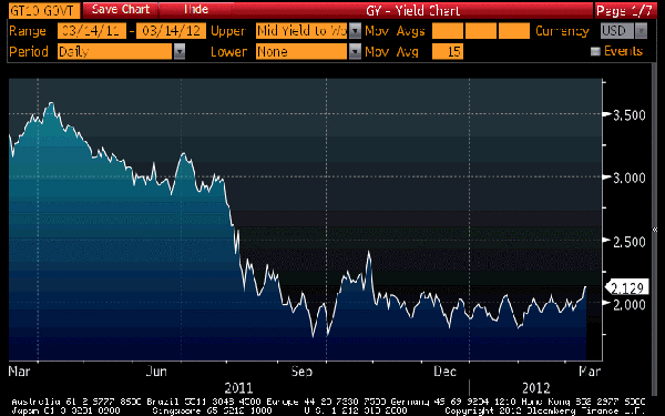
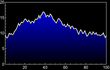
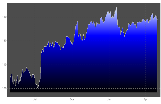
Bloomberg has a standard plot style for its line plots in which it uses a gradient filling. Actually the way this seems to be constructed is that a gradient from the ymax to ymin is used as the background in the plot area and then the area above the line is set to transparent

enter image description here.

What is the best way to make a plot like that in Mathematica for plotting {x,y} data?

$\endgroup$
4
  • 11
    $\begingroup$ An observation: the color scheme of all the parts of that plot, together, is hideously unattractive to my eyes. And having the background, above the line plot, such a dark color seems a particularly bad choice. $\endgroup$
    – murray
    Commented Mar 15, 2012 at 0:26
  • 1
    $\begingroup$ Does anyone else find it odd that a gradient oriented at right angles to this (blending left to right) is as easy as specifying ColorFunction -> (Blend[{Black, Blue}, #1] &), but a top-to-bottom blend is so complex? $\endgroup$
    – Verbeia
    Commented Mar 15, 2012 at 10:10
  • 3
    $\begingroup$ I wonder what Edward Tufte would have to say about that chart... $\endgroup$ Commented Mar 15, 2012 at 14:01
  • $\begingroup$ I guess Bloomberg never consulted Tufte. $\endgroup$ Commented Mar 15, 2012 at 20:01

9 Answers 9

30
$\begingroup$

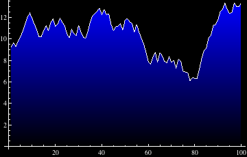
How about this?

bankerPlot[data_] := ListLinePlot[
  data,
  AxesOrigin -> {0, 0},
  Prolog -> Polygon[Join[data, Reverse[data.DiagonalMatrix[{1, 0}]]],
    VertexColors -> Join[
      Blend[{Black, Blue}, #] & /@ Normalize[data[[All, 2]], Max],
      ConstantArray[Black, Length[data]]
      ]
    ],
  PlotStyle -> White,
  Background -> Black,
  AxesStyle -> White
  ]

bankerData = Transpose[{Range[100], Accumulate[RandomReal[{-1, 1}, 100]] + 10}];
bankerPlot[bankerData]

bankerPlot output

$\endgroup$
7
  • $\begingroup$ nice one! I'll leave the question open for a little while but this looks like a winner :) $\endgroup$ Commented Mar 14, 2012 at 23:41
  • $\begingroup$ BTW in my testing I changed from Epilog to Prolog because you lose the solid line otherwise (on my system anyway) $\endgroup$ Commented Mar 14, 2012 at 23:47
  • $\begingroup$ Aha I think we caught that at about the same time. See my latest edit, 7 minutes after my first answer. $\endgroup$ Commented Mar 14, 2012 at 23:51
  • $\begingroup$ +1 for the function name (banker + plot = very sinister). $\endgroup$
    – Jens
    Commented Mar 15, 2012 at 0:27
  • $\begingroup$ I like both these methods but I find this one more intuitive than using ParametricPlot. For others it may be different. This one also seems to render faster -- not that the timings are significant enough to be a deciding factor but thought I would mention it anyway. $\endgroup$ Commented Mar 15, 2012 at 4:22
23
$\begingroup$

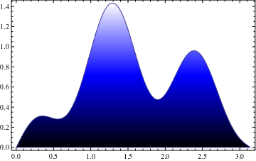
For plotting a continuous function, you could do something like this:

f[x_] := (1 + Cos[5 x]/2) Sin[x] 

ParametricPlot[{x, f[x] y}, {x, 0, Pi}, {y, 0, 1},
 PlotPoints -> 30,
 ColorFunction -> (Blend[{Black, Blue, White}, #2] &), Mesh -> None, 
 AspectRatio -> 1/GoldenRatio]

Mathematica graphics

Edit

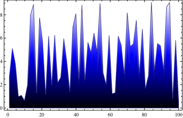
This method can be used for plotting a list of points as well by interpolating the points first, e.g.

pts1 = RandomReal[10, 100];

interpol = Interpolation[pts1, InterpolationOrder -> 1];

ParametricPlot[{x, interpol[x] y}, {x, 1, Length[pts1]}, {y, 0, 1},
 ColorFunction -> (Blend[{Black, Blue, White}, #2] &), Mesh -> None, 
 AspectRatio -> 1/GoldenRatio]

Mathematica graphics

$\endgroup$
4
  • $\begingroup$ Hi Heike, what I had in mind was for plotting {x,y} data only. $\endgroup$ Commented Mar 14, 2012 at 23:48
  • $\begingroup$ I like the edit. I can almost replicate @ArgentoSapiens except that PlotStyle->White doesn't seem to be controlling the line colour. $\endgroup$ Commented Mar 15, 2012 at 0:22
  • 2
    $\begingroup$ @MikeHoneychurch Try BoundaryStyle -> White. $\endgroup$ Commented Mar 15, 2012 at 3:48
  • $\begingroup$ @BrettChampion thanks for that. $\endgroup$ Commented Mar 15, 2012 at 4:25
19
$\begingroup$

Here's a modification of Heike's ParametricPlot approach, using textures instead of ColorFunction.

pts1 = RandomReal[10, 100];

interpol = Interpolation[pts1, InterpolationOrder -> 1];

ParametricPlot[{u, interpol[u] v}, {u, 1, Length[pts1]}, {v, 0, 1}, 
 Mesh -> None, AspectRatio -> 1/GoldenRatio, 
 TextureCoordinateFunction -> ({#1, #2} &), 
 PlotStyle -> {Opacity[1], 
   Texture[Table[{{##}} & @@ Blend[{Black, Blue, White}, 1-i], 
      {i, 0, 1, 0.01}]]}]
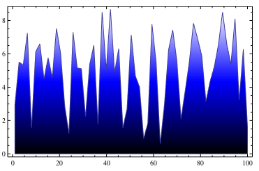
enter image description here

I'm using a 1-pixel wide Image containing the black-blue-white gradient Heike used. (Actually, it doesn't have an Image head; it's just the ImageData.)

I'm also specifying that I want the texture to correspond to the $x$ and $y$ coordinates instead of the default of $u$ and $v$.

This approach allows us to generalize the gradient to something more complicated, or even an arbitrary image:

ParametricPlot[{u, interpol[u] v}, {u, 1, Length[pts1]}, {v, 0, 1}, 
 Mesh -> None, AspectRatio -> 1/GoldenRatio, 
 TextureCoordinateFunction -> ({#1, #2} &), 
 PlotStyle -> {Opacity[1], Texture[ExampleData[{"TestImage", "Lena"}]]}]
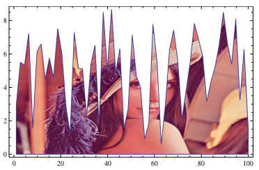
enter image description here

$\endgroup$
1
  • $\begingroup$ Thanks Brett. I can see where I might want to use this with country's flag as a texture. $\endgroup$ Commented Mar 15, 2012 at 4:28
17
$\begingroup$

This is a variant of Argento's answer with the blend on a rectangle in the background rather than creating a polygon that matches the data.

bankerData = 
  Transpose[{Range[100], Accumulate[RandomReal[{-1, 1}, 100]] + 10}];


ListLinePlot[bankerData, Frame -> True, Background -> Black, 
 AxesOrigin -> {0, 0}, PlotRange -> {{1, 100}, {0, 20}}, 
 FrameTicks -> {{Automatic, None}, {Automatic, None}}, 
 PlotRangePadding -> 0, 
 BaseStyle -> {Thick, White, FontFamily -> "Arial", FontSize -> 13}, 
 Filling -> Top, FillingStyle -> Black, Mesh -> None, 
 PlotStyle -> Directive[Thick, White], 
 Prolog -> 
  Polygon[{Scaled[{0, 0}], Scaled[{1, 0}], Scaled[{1, 1}], 
    Scaled[{0, 1}]}, VertexColors -> {Black, Black, Blue, Blue}]]

enter image description here

The disadvantage of my approach is that you need to set PlotRangePadding->0.

$\endgroup$
2
  • $\begingroup$ hmmm, I like this one the best now :). I usually set PlotRangePadding->0 by default anyway so that would not be an issue for me. $\endgroup$ Commented Mar 15, 2012 at 19:59
  • $\begingroup$ @Verbeia, blue artifacts appear when trying to migrate the model to DateListPlot (to take advantage of FinancialData. koStock = FinancialData["KO", {2013, 1, 1}]; DateListPlot[koStock, AxesOrigin -> {First@koStock[[All, 1]], 0}, Frame -> True, Background -> Black, BaseStyle -> {Thick, White, FontFamily -> "Arial", FontSize -> 13}, Filling -> Top, FillingStyle -> Black, Mesh -> None, PlotStyle -> Directive[Thick, White], Prolog -> Polygon[{Scaled[{0, 0}], Scaled[{1, 0}], Scaled[{1, 1}], Scaled[{0, 1}]}, VertexColors -> {Black, Black, Blue, Blue}], PlotRangePadding -> 0] $\endgroup$
    – Zviovich
    Commented Jan 10, 2014 at 14:46
14
$\begingroup$

Here is another method that uses the more general gradient background construction I posted as an answer to "How can I set different opacity values for the background of a ListPlot".

This answer is rather late, but I thought it's a good example of how else to use the simple option Prolog -> gradientBackground to create a gradient background:

gradientBackground = 
  With[{bottomColor = Black, topColor = Lighter[Blue]}, 
   Inset[Show[
     Rasterize[
      Graphics[
       Polygon[{{0, 0}, {1, 0}, {1, 1}, {0, 1}}, 
        VertexColors -> {bottomColor, bottomColor, topColor, 
          topColor}], PlotRangePadding -> 0, ImagePadding -> 0], 
      "Image"], AspectRatio -> Full], {Left, Bottom}, {0, 0}, 
    ImageScaled[{1, 1}]]];


bankerData = 
  Transpose[{Range[100], Accumulate[RandomReal[{-1, 1}, 100]] + 10}];

ListLinePlot[
 bankerData,
 Prolog -> gradientBackground,
 PlotRangePadding -> None,
 Frame -> True,
 Axes -> False,
 GridLines -> Automatic,
 PlotStyle -> White,
 FrameLabel -> {"x", "y"},
 Method -> {"GridLinesInFront" -> True},
 PlotRegion -> {{.04, .96}, {.04, .96}},
 Background -> Black,
 Filling -> Top,
 FillingStyle -> Black,
 PlotRange -> All,
 BaseStyle -> {White, FontFamily -> "Arial"}]

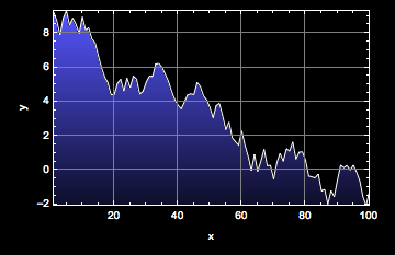
banker plot

$\endgroup$
10
$\begingroup$

If you can accept the limitation of a two-color gradient here is another option:

bankerData = 
  Transpose[{Range[100], Accumulate[RandomReal[{-1, 1}, 100]] + 10}];

p1 = ListLinePlot[
       bankerData, 
       ColorFunction -> ({Black, Red} ~Blend~ #2 &),
       Filling -> Axis
     ];

n = Length @ bankerData;

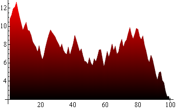
MapAt[Join[# ~Take~ n, Black & /@ # ~Drop~ n] &, p1, {1, -1, 2}]

Mathematica graphics

The index {1, -1, 2} is for the VertexColors list. It works on version 7. If it does not work on your version either find the right index, or use patterns, e.g.:

pos = {#, #2, 2} & @@ Position[p1, VertexColors][[-1]];

MapAt[Join[#~Take~n, Black & /@ #~Drop~n] &, p1, pos]
$\endgroup$
10
$\begingroup$

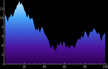
While trying to force ColorFunction to work I came up with this:

bankerData = Transpose[{Range[100], Accumulate[RandomReal[{-1, 1}, 100]] + 10}];

bands = 20;

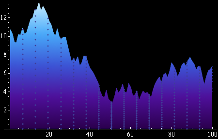
ListLinePlot[Table[{1, i} # & /@ bankerData, {i, 0`, 1`, 1/bands}], 
 Background -> Black, AxesStyle -> White, 
 ColorFunction -> "DeepSeaColors", 
 Filling -> True
]

enter image description here

Adding Mesh -> True gives an idea of how it works:

enter image description here

$\endgroup$
8
$\begingroup$

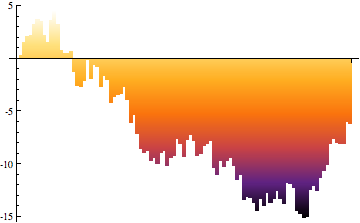
If you are willing to consider a bar chart instead, this can be done with sufficient segments in a "SegmentScaleRectangle" setting for ChartElementFunction. Rendering is a little slow but the result is quite attractive.

testdata = 
  FoldList[0.99 #1 + #2 &, 0., 
   RandomVariate[NormalDistribution[0, 1], 100]];

BarChart[testdata, ChartStyle -> EdgeForm[None], BarSpacing -> 0, 
 PerformanceGoal -> "Speed", 
 ChartElementFunction -> 
  ChartElementDataFunction["SegmentScaleRectangle", "Segments" -> 200,
    "ColorScheme" -> "SunsetColors"]]

enter image description here

This works fine with dark backgrounds: all one needs to do is add
BaseStyle -> White, Background->Black to the options in the BarChart or RectangleChart.

$\endgroup$
3
$\begingroup$

New-in-version-12.2.0 styling directive LinearGradientFilling makes the task more straightforward:

data = FinancialData["IBM", "OHLCV", {{2009, 5, 1}, {2010, 4, 30}}]; 

DateListPlot[data["PathComponent", 4], 
 PlotStyle -> Directive[Thin, GrayLevel[.7]], PlotMarkers -> None, 
 Filling -> Axis, 
 FillingStyle ->
    LinearGradientFilling[{Black, Darker@Darker@Blue, Blue, LightBlue},  Top], 
 PlotTheme -> "Marketing", 
 GridLinesStyle -> Directive[GrayLevel[.4], Dashed], 
 Method -> {"GridLinesInFront" -> True}, ImageSize -> Large] 

enter image description here

$\endgroup$

Your Answer

By clicking “Post Your Answer”, you agree to our terms of service and acknowledge you have read our privacy policy.

Not the answer you're looking for? Browse other questions tagged or ask your own question.