Most concise code for tangent and normal line of implicit algebraic curve

Question

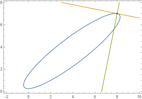
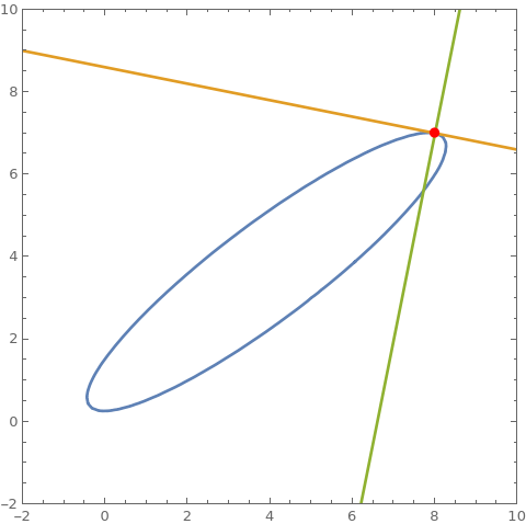
Can you make the code for tangent line and normal line of implicit algebraic curve cu more concise than mine?

The code for tangent line at {x,y}={8,7} is:

D[cu, {{x, y}}] . {a - x, b - y} /. {x -> 8, y -> 7} /. {a -> x, b -> y} // Expand

The code for normal line at {x,y}={8,7} is:

D[cu, {{y, x}}] . {a - x, -b + y} /. {x -> 8, y -> 7} /. {a -> x, b -> y} // Expand

What I do not like about my code is that it uses two Rule's and two temporary and meaningless variables a, b.

cu = 3 x^2 + 5 y^2 - 7 x y + 2 x - 9 y + 2;
cu == 0 /. {x -> 8, y -> 7}
D[cu, {{x, y}}] . {a - x, b - y} /. {x -> 8, y -> 7} /. {a -> x, 
   b -> y} // Expand
D[cu, {{y, x}}] . {a - x, -b + y} /. {x -> 8, y -> 7} /. {a -> x, 
   b -> y} // Expand
ContourPlot[{cu == 0, %% == 0, % == 0}, {x, -2, 10}, {y, 0, 8}, 
 Epilog -> {Point[{8, 7}]}, AspectRatio -> Automatic]
Clear[cu]

(* True *)

(* -43 + x + 5 y *)

(* -33 + 5 x - y *)

Answer 1

• For the curve f[x,y]==0, we use

grad = Through@*Apply[{Derivative[1, 0][f], Derivative[0, 1][f]}];

to define a Grad operator to calculus the normal of implicit curve f[x,y]==0 on the point pt={a,b}={8,7}.

Clear["Global`*"];
f[x_, y_] := 3 x^2 + 5 y^2 - 7 x y + 2 x - 9 y + 2;
rotation = RotationTransform[π/2];
grad = Through@*Apply[{Derivative[1, 0][f], Derivative[0, 1][f]}];
pt = {8, 7};

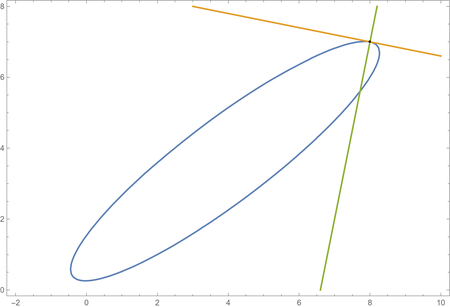
ContourPlot[{f[x, y] == 0, grad@{a, b} . {x - a, y - b} == 0, 
    rotation@grad@{a, b} . {x - a, y - b} == 0} /. 
   Thread[{a, b} -> pt] // Evaluate, {x, -2, 10}, {y, 0, 8}, 
 Epilog -> {Point[pt]}, AspectRatio -> Automatic]

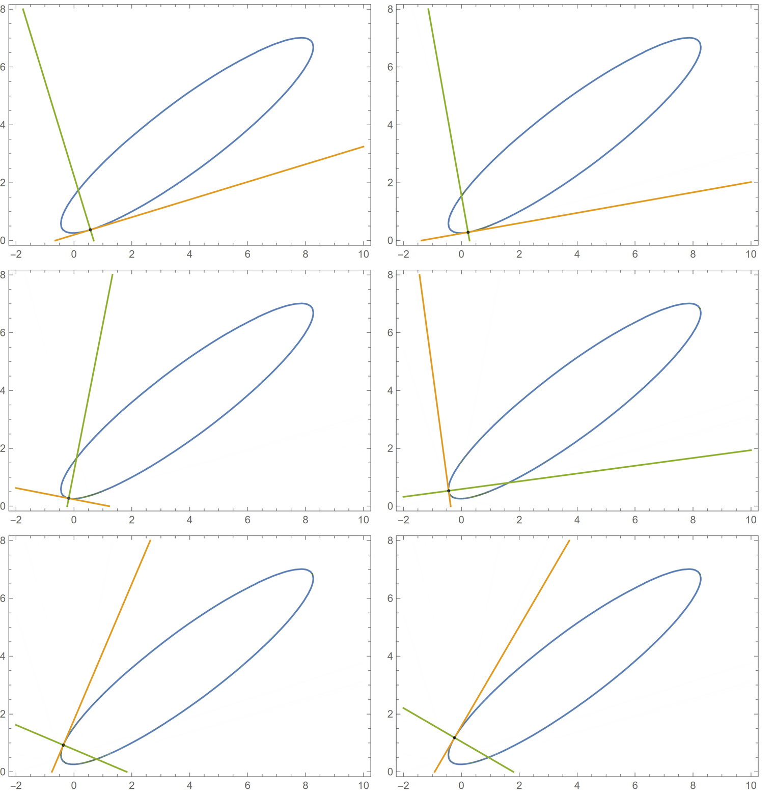
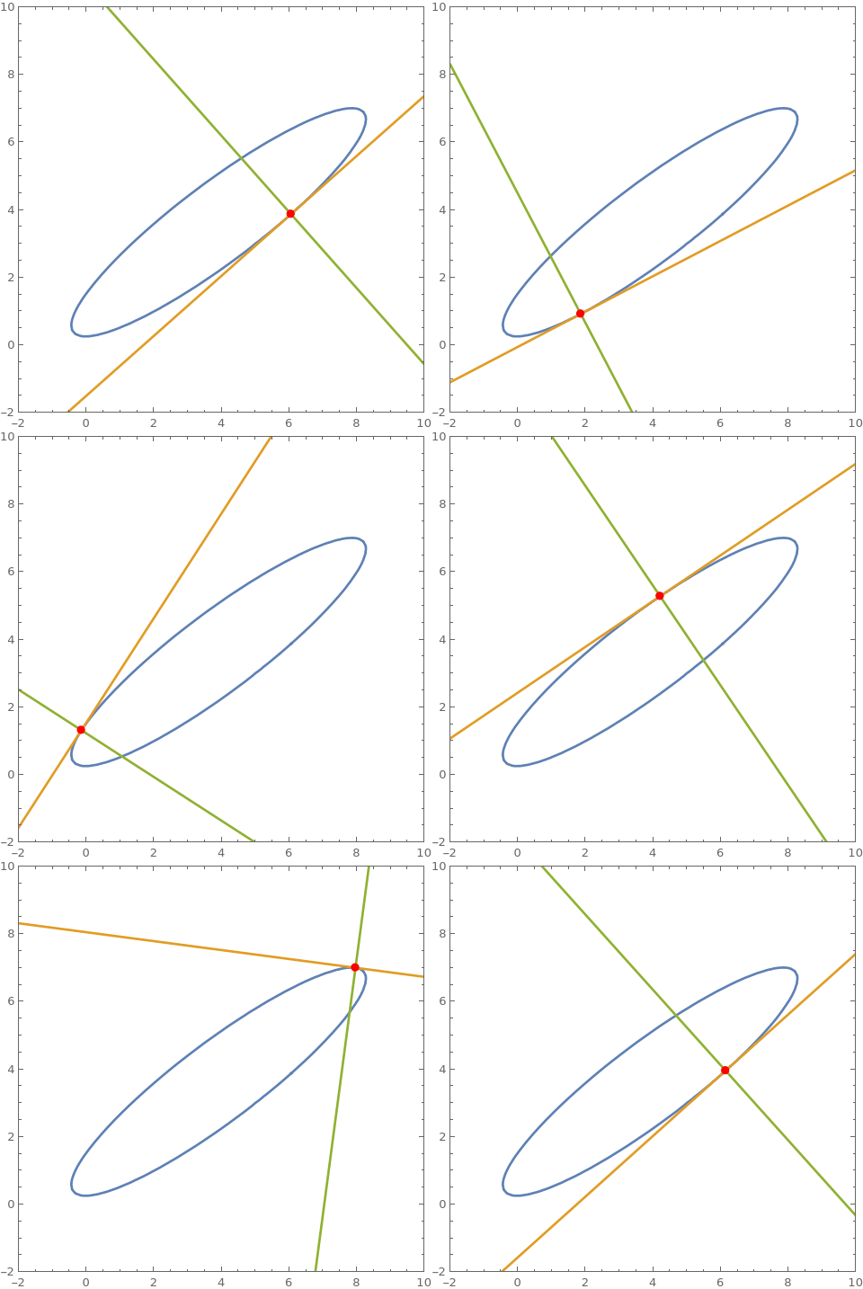
• animation.

plot = ContourPlot[f[x, y] == 0, {x, -2, 10}, {y, 0, 8}];
pts = Cases[plot, GraphicsComplex[pts_, data__] :> pts, -1] // First;
data = Table[
   ContourPlot[{f[x, y] == 0, grad@pt . ({x, y} - pt) == 0, 
      rotation@grad@pt . ({x, y} - pt) == 0} // Evaluate, {x, -2, 
     10}, {y, 0, 8}, Epilog -> {Point[pt]}, 
    AspectRatio -> Automatic], {pt, pts}];
ani = ListAnimate[data]

Answer 2

You can useDt. For example for curve cu:

cu = 3 x^2 + 5 y^2 - 7 x y + 2 x - 9 y + 2;

you can do:

tn[f_, p_] := Module[{td = Dt[f], t, n, ex1, ex2},
  t = td /. {Dt[x] -> {1, 0}, Dt[y] -> {0, 1}};
  n = td /. {Dt[x] -> {0, 1}, Dt[y] -> {-1, 0}};
  ex1 = (t /. Thread[{x, y} -> p]) . ({x, y} - p);
  ex2 = (n /. Thread[{x, y} -> p]) . ({x, y} - p);
  Column[{ContourPlot[{f == 0, ex1 == 0, ex2 == 0}, {x, -2, 
      10}, {y, -2, 10}, Epilog -> {Red, Point[p]}],
    Grid[{{"curve", f == 0}, {StringForm["tangent at ``", p], 
       ex1 == 0},
      {StringForm["normal at ``", p], ex2 == 0}}, Alignment -> Left, 
     Frame -> All, ItemSize -> 30]
    }, Frame -> All]]

Note the first 4 lines are relevant. The rest is window dressing for visualization.

Using @cvgmt pts: pts = Cases[ContourPlot[cu == 0, {x, -2, 10}, {y, -2, 10}], GraphicsComplex[pts_, data__] :> pts, -1] // First;

and exporting as animated gif:

Answer 3

One alternative:

curve = 3 x^2 + 5 y^2 - 7 x y + 2 x - 9 y + 2; {$x, $y} = {8, 7};
slope = D[curve, x]/D[curve, y] /. {x -> $x, y -> $y};
{tangent, orthogonal} =  (y - $y) + # (x - $x) slope^# & /@ {1, -1};

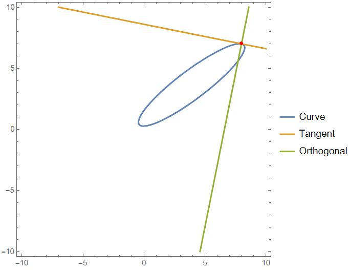
ContourPlot[{curve == 0, tangent == 0, orthogonal == 0}
   , {x,-10,10}, {y, -10, 10}
   , PlotLegends -> {"Curve", "Tangent", "Orthogonal"}
   , Epilog -> {Red, PointSize -> Medium, Point[{$x, $y}]}
, AspectRatio -> Automatic]

Answer 4

{$tF, $nF} = Table[With[{i = i}, 
  Module[{v = Variables[#]}, Dot[i @ Grad[#, v] /. Thread[v -> #2], v - #2]] &],
 {i, {Identity, Cross}}];

Examples:

cu = 2 + 2 x + 3 x^2 - 9 y - 7 x y + 5 y^2;

pt = {8, 7};

ContourPlot[Evaluate @ {cu == 0, $tF[cu, pt] == 0, $nF[cu, pt]}, 
 {x, -2, 10}, {y, -2, 10}, 
 PlotRange -> {{-2, 10}, {-2, 10}}, 
 Epilog -> {Red  , PointSize @ Large, Point @ pt}]

cP[pt_] := ContourPlot[
  Evaluate @ {cu == 0, tLF[cu, pt] == 0, nLF[cu, pt]}, 
  {x, -2, 10}, {y, -2, 10}, 
  PlotRange -> {{-2, 10}, {-2, 10}}, 
  Epilog -> {Red  , PointSize@Large, Point@pt}];

coords = First @ Cases[ContourPlot[cu == 0, {x, -2, 10}, {y, -2, 10}], 
   GraphicsComplex[c_, ___] :> c, All];

frames = cP /@ coords;

Export["tnframes.gif", frames[[;; ;; 2]], DisplayAllSteps -> True]

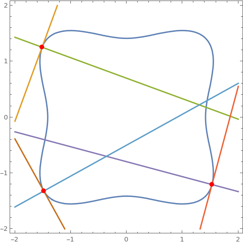
cu2 = x^4 - 2 x^2 + y^4 - 2 y^2;

SeedRandom[1];
pts = RandomSample[{x, y} /. FindInstance[cu2 == 0, {x, y}, Reals, 20], 3];

ContourPlot[Evaluate @ 
    {cu2 == 0, 
     $tL[cu2, pts[[1]]] == 0, $nL[cu2, pts[[1]]] == 0, 
     $tL[cu2, pts[[2]]] == 0, $nL[cu2, pts[[2]]] == 0,
     $tL[cu2, pts[[3]]] == 0, $nL[cu2, pts[[3]]] == 0},
   {x, -2, 2}, {y, -2, 2}, 
  Epilog -> {Red  , PointSize@Large, Point /@ pts}]

Answer 5

A concise form of the tangent line can be obtained with homogeneous coordinates (HC). In HC the ellipse is implicitly written:

m = {{2, 1, -9/2}, {1, 3, -7/2}, {-9/2, -7/2, 5}};
p = {1, x, y};
p.m.p==0

2 + 2 x + 3 x^2 - 9 y - 7 x y + 5 y^2 ==0

This is the same formula as your cu==0

Now the formula for the tangent at {8,7} can be written very simply:

p0={1,8,7};
p0.m.p == 0

As this are homogeneous coordinates, this is the same line as:

-43 + x + 5 y == 0

The normal to a line given by: {a0,a1,a2} through the point {1,b1,b2} on a is:

 {-a1 b2+a2 b1,- a2,a1}

and the equation of this line:

-a1 b2+a2 b1 - a2 x + a1 y ==0

Therefore for your case:

{-1 7 + 5 8, -5, 1} -> {3,-5,1}

resulting in the normal equation:

33 - 5 x + y == 0