4
$\begingroup$
DamOne4u25jul2023 = {{-3., 52.769}, {-2., 52.769}, {-1., 52.769}, {0., 52.769}, {0.583417, 52.442}, {1.63294, 52.585}, {2.05024, 52.248}, {3.02856, 50.69}, {3.70292, 50.353}, {4.6758, 50.268}, {5.12138, 49.98}, {5.69973, 49.97}, {6.26108, 49.793}, {6.81076, 49.808}, {7.28225, 49.849}, {7.8346, 49.89}, {8.3223, 49.916}, {8.89531, 49.97}, {9.38787, 50.018}, {9.96094, 50.131}, {10.405, 50.225}, {10.9097, 50.226}, {11.3754, 50.216}, {11.9463, 50.192}, {12.4333, 50.108}, {12.9852, 50.069}, {13.4489, 50.102}, {14.064, 50.122}, {14.5248, 50.157}, {15.0122, 50.146}, {15.5716, 50.276}, {16.1521, 50.402}, {16.6409, 50.789}, {17.1445, 50.797}, {17.4839, 50.989}, {18.1874, 51.077}, {18.6137, 51.153}, {19.1646, 51.313}, {20.0555, 51.573}, {20.1036, 52.39}, {20.4138, 52.773}, {20.7461, 53.579}, {21., 53.579}, {22., 53.579}, {23., 53.579}}
SpDamOne4u25jul2023 = Interpolation[DamOne4u25jul2023, Method -> "Spline", InterpolationOrder -> 3] 
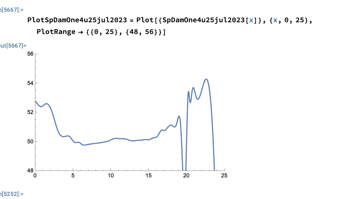
PlotSpDamOne4u25jul2023 = Plot[{SpDamOne4u25jul2023[x]}, {x, 0, 25}, PlotRange -> {{0, 25}, {48, 56}}]

The points given in my actual code are not hard coded: it's an Import from an excel file. Additionally, the project I'm working on has years of previous creek cross sections that are graphed properly by a 3rd order spline function. The goal is to show the change in elevation of the creek's floor.

I had two ideas of how to rectify this issue;

  1. Add buffer points where the data is struggling to fit the curve so that it will avoid the large dip and to possibly guide the cubic line.
  2. I could change the InterpolationOrder to 1, but for the goal of the project I'm working on keeping the Order as 3 is more desirable.

This is the output of the graph, the large dip on the right end reaches a minimum of 47, the data set the spline function is graphing has a minimum of 49.

$\endgroup$
2
  • 3
    $\begingroup$ Splines consist of polynomials. In fitting points, polynomiales will always overshoot if the slope changes rapidly. $\endgroup$ Commented Aug 9, 2023 at 14:24
  • 1
    $\begingroup$ Try spDamOne4u25jul2023 = ResourceFunction["CubicMonotonicInterpolation"][damOne4u25jul2023], though it's not much different from linear interpolation. Anyway, it shows cubic polynomials do not have to overshoot. You should generally ignore the plot for $x > 23$, for which function values are extrapolated. Extrapolation tends to diverge from the trend of the data, unless the polynomial interpolant is a good model for the underlying process, which is almost never the case. Related: mathematica.stackexchange.com/a/140386, mathematica.stackexchange.com/a/11859/4999. $\endgroup$
    – Michael E2
    Commented Aug 9, 2023 at 14:37

1 Answer 1

5
$\begingroup$

Sometimes it helps to evenly space your data before interpolation: Let's first look at the successive spacings between your data points:

Differences[DamOne4u25jul2023[[All, 1]]]

{1., 1., 1., 0.583417, 1.04952, 0.4173, 0.97832, 0.67436, 0.97288, \ 0.44558, 0.57835, 0.56135, 0.54968, 0.47149, 0.55235, 0.4877, \ 0.57301, 0.49256, 0.57307, 0.44406, 0.5047, 0.4657, 0.5709, 0.487, \ 0.5519, 0.4637, 0.6151, 0.4608, 0.4874, 0.5594, 0.5805, 0.4888, \ 0.5036, 0.3394, 0.7035, 0.4263, 0.5509, 0.8909, 0.0481, 0.3102, \ 0.3323, 0.2539, 1., 1.}

We see some are close to 1, some are spaced 0.5 units apart, others close to 0.25 units, etc.

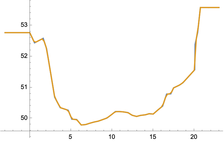
Let's just try and linearly interpolate first to grab values for the creek bed at every 0.25 units (this is not our overall interpolation yet, we're just using it to grab evenly spaced values). Let's also validate our evenly spaced data by plotting it with our original dataset:

int1 = Interpolation[DamOne4u25jul2023, InterpolationOrder -> 1]
evenSpacedData = Table[{x, int1[x]}, {x, Range[-3, 23, 0.25]}];
ListLinePlot[{DamOne4u25jul2023, evenSpacedData}]

enter image description here

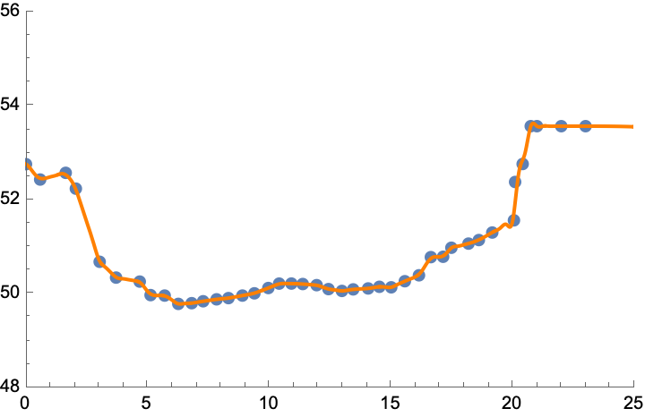
Indeed we see they are quite similar. Now we can use a cubic spline interpolation with our evenly spaced data, and the troublesome dips and spikes are gone!

newSpline = 
 Interpolation[evenSpacedData, Method -> "Spline", InterpolationOrder -> 3];

splinePlot = 
  Plot[{newSpline[x]}, {x, 0, 25}, PlotRange -> {{0, 25}, {48, 56}}, 
  PlotStyle -> Orange];

Show[ListPlot[DamOne4u25jul2023, PlotRange -> {{0, 25}, {48, 56}}, 
  PlotMarkers -> Automatic], splinePlot]

enter image description here

$\endgroup$
1
  • $\begingroup$ I like this. For what it's worth, experimentally just removing {20.4138, 52.773} already seems to help for the original setup. $\endgroup$ Commented Aug 9, 2023 at 20:37

Your Answer

By clicking “Post Your Answer”, you agree to our terms of service and acknowledge you have read our privacy policy.

Not the answer you're looking for? Browse other questions tagged or ask your own question.