To use "RowReduce" to solve linear equations you must append the RHS as an additional column to your matrix. The solution is then the rightmost column of the matrix in reduced row echelon form.
Here is an example:
Given the system of 3 linear equations:
a = {{2, 3, 5}, {-3, 4, -1}, {4, 1, -6}};
b = {-2, 7, 3};
Thread[a . {x, y, z} == b] // MatrixForm

We must append the RHS as column to the right side of a:
MatrixForm[m = Join[a, Transpose[{b}], 2]]

The rightmost column of the row reduced matrix is now the solution:
(m1 = RowReduce[m]) // MatrixForm

We can test this:
m1[[All, 4]] == {x, y, z} /. Solve[a . {x, y, z} == b]
(* True *)
Addendum
Now what happens if the row are not linearly independent or if the system is over determined?
For the case where the rows are linearly depended, We replace the third row by the sum of the first and twice the second row:
m2 = m; m2[3] = m[1] + 2 m[2];
(m3 = RowReduce[m2]) // MatrixForm

The last row is all zeros. Telling us that there is no unique solution. The first 2 rows give 2 equations for 3 variable, leaving one variable free.
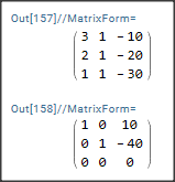
For an over determined system, it may have a solution or not. For the case that there exists a solution {-10,40}, consider:
m = {{3, 1, -b1}, {2, 1, -b2}, {1, 1, -b3}};
(m1 = m /. {b1 -> 10, b2 -> 20, b3 -> 30}) // MatrixForm
(m2 = RowReduce[m1]) // MatrixForm

There is no problem, we get the correct solution.
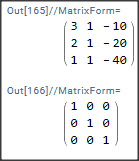
But what if the system is inconsistent? For this we change b3 from 30 to 40:
(m1 = m /. {b1 -> 10, b2 -> 20, b3 -> 40}) // MatrixForm
(m2 = RowReduce[m1]) // MatrixForm

What does this tell us? Remember that the rightmost columns are the RHS of our equation And this is means:
m2.{x,y,1}== {0,0,0}
Therefore the last row tells us 1 == 0, a contradiction. This indicates that the system has no solution.
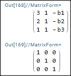
Now hat happens if b is symbolic? Let see:
m // MatrixForm
RowReduce[m] // MatrixForm

Obviously MMA assumes that the system is inconsistent.


