3
$\begingroup$

The following transient problem is essentially the reciprocating (i.e., fully reversing) flow of a fluid over a thick heated block until the system reaches a cyclic steady-state (i.e., the system temperature oscillates around a mean when this point is reached). The following code simulates the system for a fluid velocity boundary condition $u=3*\sin(2*\pi*0.5*t)$, i.e., a frequency of $0.5Hz$ and a heat flux input of $1000 W/m^2$. tflow refers to the total time till which the flow oscillation occurs and t0 is the time-step. The code uses the flow solver developed by Alex Trounev and described in this page.

Needs["NDSolve`FEM`"]

{f = 0.5; L = 0.040, d = 0.003, e = 0.005, kf = 0.026499, ks = 16, 
 rho = 1.1492, rhos = 7860, mu = 18.923*10^-6, cp = 1.0069*10^3, 
 cps = 502.4}; u0 = 3; nu = mu/rho; om = 2 Pi f;
tflow = 400;
t0 = .3;
NV = 2 f tflow;
nn = Round[NV \[Pi]/(om t0)]
Ti = 307; q = 1000/Ti;

reg1 = ImplicitRegion[0 <= x <= L && 0 <= y <= d, {x, y}]; reg2 = 
 ImplicitRegion[0 <= x <= L && -e <= y <= d, {x, y}];
UX[0][x_, y_] := 0;
VY[0][x_, y_] := 0;
P[0][x_, y_] := 0;
Tfs[0][x_, y_] := 307/Ti; appro = 
 With[{k = 2. 10^6}, ArcTan[k #]/Pi + 1/2 &];
ade[y_] := (ks + (kf - ks) appro[y])
rde[y_] := (cps rhos + (cp rho - cps rhos) appro[y]);

Monitor[Do[{UX[i], VY[i], P[i]} = 
    NDSolveValue[{{Inactive[
            Div][({{-\[Mu], 0}, {0, -\[Mu]}}.Inactive[Grad][
              u[x, y], {x, y}]), {x, y}] + D[p[x, y], x] + 
          UX[i - 1][x, y]*D[u[x, y], x] + 
          VY[i - 1][x, y]*D[u[x, y], y] + (u[x, y] - UX[i - 1][x, y])/
           t0, Inactive[
            
            Div][({{-\[Mu], 0}, {0, -\[Mu]}}.Inactive[Grad][
              v[x, y], {x, y}]), {x, y}] + D[p[x, y], y] + 
          UX[i - 1][x, y]*D[v[x, y], x] + 
          VY[i - 1][x, y]*D[v[x, y], y] + (v[x, y] - VY[i - 1][x, y])/
           t0, D[u[x, y], x] + D[v[x, y], y]} == {0, 0, 0} /. \[Mu] ->
         nu, {DirichletCondition[{u[x, y] == u0*Sin[om*i*t0], 
         v[x, y] == 0}, 
        x == L (1 - Sign[Sin[om*i*t0]])/2 && 0 < y < d], 
       DirichletCondition[{u[x, y] == 0, v[x, y] == 0}, 
        y == 0 || y == d]}, 
      DirichletCondition[p[x, y] == 0, 
       x == L (1 + Sign[Sin[om*i*t0]])/2 && 0 < y < d]}, {u, v, 
      p}, {x, y} \[Element] reg1, 
     Method -> {"FiniteElement", 
       "InterpolationOrder" -> {u -> 2, v -> 2, p -> 1}, 
       "MeshOptions" -> {"MaxCellMeasure" -> 0.0000005}}];
   ux = If[y <= 0, 0, UX[i][x, y]]; vy = If[y <= 0, 0, VY[i][x, y]];
   Tfs[i] = 
    NDSolveValue[{rde[
           y] ((ux*D[T[x, y], x] + 
              vy*D[T[x, y], y]) + (T[x, y] - Tfs[i - 1][x, y])/t0) - 
         Inactive[Div][
          ade[y]*Inactive[Grad][T[x, y], {x, y}], {x, y}] == 
        NeumannValue[q, y == -e], 
       DirichletCondition[{T[x, y] == 1}, 
        x == L (1 - Sign[Sin[om*i*t0]])/2 && 0 <= y <= d]}, 
      T, {x, y} \[Element] reg2, 
      Method -> {"FiniteElement", "InterpolationOrder" -> {T -> 2}, 
        "MeshOptions" -> {"MaxCellMeasure" -> 0.0000001}}] // 
     Quiet;, {i, 1, nn}],ProgressIndicator[i,{1,nn}]]; // AbsoluteTiming

ListLinePlot[
 Table[{i t0, Tfs[i][0.5*L, -e/2]*Ti - 273.16}, {i, 0, nn}], 
 AxesLabel -> {"t(s)", "T(in deg. C)"}, PlotRange -> Full]

If one plots the temperature profile at a point $(0.5L,-e/2)$ in the solid with time, it turns out to be: enter image description here
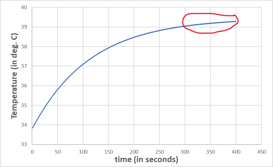
As can be seen, the temperature of the system initially increases fast to gradually slow down and reach a cyclic steady-state (marked with red), where it oscillates around a mean.

However, keeping all other parameters same, if I increase the frequency to say f=2 Hz, I need to give a smaller time-step which should be at-least $<\frac{1}{2*2}=0.25s$, to resolve the flow reversal in each half-period correctly. In this scenario, the tflow required to reach a cyclic steady-state increases.

When I run the above code with f=2, t0=0.1,tflow=800, it crashes each and every time with the error Wolfram Kernel has stopped working. My question is:

  1. Can this code be improved so that it does not crash for high f, which require small t0? For example: f=2, t0=0.1
$\endgroup$
2

1 Answer 1

5
$\begingroup$

To answer first question we can improve code by separating fluid part and using mesh with QuadElement only as follows

Needs["NDSolve`FEM`"]
{f = 2;
 L = 0.040, d = 0.003, e = 0.005, kf = 0.026499, ks = 16, 
 rho = 1.1492, rhos = 7860, mu = 18.923*10^-6, cp = 1.0069*10^3, 
 cps = 502.4}; u0 = 3; nu = mu/rho; om = 2 Pi f;
tflow = 800;
t0 = .1;
NV = 2 f tflow;
nn = Round[NV \[Pi]/(om t0)]
Ti = 307; q = 1000/Ti;

reg1 = ImplicitRegion[0 <= x <= L && 0 <= y <= d, {x, y}]; reg2 = 
 ImplicitRegion[0 <= x <= L && -e <= y <= d, {x, y}];

mesh = ToElementMesh[FullRegion[2], {{0, L}, {0, d}}];
mesh1 = ToElementMesh[FullRegion[2], {{0, L}, {-e, d}}];
UX[0][x_, y_] := 0;
VY[0][x_, y_] := 0;
P[0][x_, y_] := 0;
Tfs[0][x_, y_] := 307/Ti; appro = 
 With[{k = 2. 10^6}, ArcTan[k #]/Pi + 1/2 &];
ade[y_] := (ks + (kf - ks) appro[y])
rde[y_] := (cps rhos + (cp rho - cps rhos) appro[y]);
eqs = {Inactive[
     Div][({{-\[Mu], 0}, {0, -\[Mu]}} . 
      Inactive[Grad][u[x, y], {x, y}]), {x, y}] + D[p[x, y], x] + 
   UX[i - 1][x, y]*D[u[x, y], x] + 
   VY[i - 1][x, y]*D[u[x, y], y] + (u[x, y] - UX[i - 1][x, y])/t0, 
  Inactive[
     Div][({{-\[Mu], 0}, {0, -\[Mu]}} . 
      Inactive[Grad][v[x, y], {x, y}]), {x, y}] + D[p[x, y], y] + 
   UX[i - 1][x, y]*D[v[x, y], x] + 
   VY[i - 1][x, y]*D[v[x, y], y] + (v[x, y] - VY[i - 1][x, y])/t0, 
  D[u[x, y], x] + D[v[x, y], y]}; 
bc[i_] := {DirichletCondition[{u[x, y] == u0*Sin[om*i*t0], 
    v[x, y] == 0}, x == L (1 - Sign[Sin[om*i*t0]])/2 && 0 < y < d], 
  DirichletCondition[{u[x, y] == 0, v[x, y] == 0}, y == 0 || y == d], 
  DirichletCondition[p[x, y] == 0, 
   x == L (1 + Sign[Sin[om*i*t0]])/2 && 0 < y < d]};

Monitor[Do[{UX[i], VY[i], P[i]} = 
      NDSolveValue[{eqs == {0, 0, 0} /. \[Mu] -> nu, bc[i]}, {u, v, 
        p}, {x, y} \[Element] mesh, 
       Method -> {"FiniteElement", 
         "InterpolationOrder" -> {u -> 2, v -> 2, p -> 1}}];, {i, 1, 
     nn}], ProgressIndicator[i, {1, nn}]]; // AbsoluteTiming

It takes about 1871s on my laptop. Visualization last 20 frames

Table[DensityPlot[UX[i][x, y], {x, y} \[Element] mesh, 
  ColorFunction -> "Rainbow", PlotRange -> All, 
  AspectRatio -> Automatic, Frame -> False], {i, nn - 19, nn}]

Figure 1

With this velocity field we can compute temperature as follows

Monitor[Do[ux = If[y <= 0, 0, UX[i][x, y]]; 
    vy = If[y <= 0, 0, VY[i][x, y]];
    Tfs[i] = 
     NDSolveValue[{rde[
            y] ((ux*D[T[x, y], x] + 
               vy*D[T[x, y], y]) + (T[x, y] - Tfs[i - 1][x, y])/t0) - 
          Inactive[Div][
           ade[y]*Inactive[Grad][T[x, y], {x, y}], {x, y}] == 
         NeumannValue[q, y == -e], 
        DirichletCondition[{T[x, y] == 1}, 
         x == L (1 - Sign[Sin[om*i*t0]])/2 && 0 <= y <= d]}, 
       T, {x, y} \[Element] mesh1, 
       Method -> {"FiniteElement", 
         "InterpolationOrder" -> {T -> 2}}] // Quiet;, {i, 1, nn}], 
   ProgressIndicator[i, {1, nn}]]; // AbsoluteTiming

It takes about 1086s. Visualization

{ListLinePlot[
  Table[{i t0, Tfs[i][0.5*L, -e/2]*Ti - 273.16}, {i, 0, nn}], 
  AxesLabel -> {"t(s)", "T(in deg. C)"}, PlotRange -> Full], 
 ListLinePlot[
  Table[{i t0, Tfs[i][0.5*L, -e/2]*Ti - 273.16}, {i, nn - 40, nn}], 
  AxesLabel -> {"t(s)", "T(in deg. C)"}, PlotRange -> Full]}

Figure 2

$\endgroup$
5
  • $\begingroup$ Thankyou for these modifications. Right now I am running a example and it has not crashed till now. I am optimistic that this has done the trick. $\endgroup$
    – Avrana
    Commented Dec 13, 2022 at 5:50
  • $\begingroup$ I ran the code for f=2, tflow=1000, q=5000/Ti. It took a total of 8hr 51min to execute on my 8-core AMD Ryzen 7 5800H laptop. But it did not crash. This solution surely answers the first question. I will accept it in a day if no answer to the second part is forthcoming. Thankyou again Alex. $\endgroup$
    – Avrana
    Commented Dec 14, 2022 at 4:50
  • 1
    $\begingroup$ @Avrana It could be better to ask second question in separate post. Since answer is not simple. There are several papers about this problem as I remember from discussion on mathematica.stackexchange.com/questions/262999/… $\endgroup$ Commented Dec 14, 2022 at 5:53
  • $\begingroup$ I think you are right. I have accepted the answer and will post a separate question for the second part. $\endgroup$
    – Avrana
    Commented Dec 14, 2022 at 6:17
  • $\begingroup$ I have posted a separate question here. $\endgroup$
    – Avrana
    Commented Dec 15, 2022 at 6:53

Your Answer

By clicking “Post Your Answer”, you agree to our terms of service and acknowledge you have read our privacy policy.