How can I manipulate multiple functions which all have the same parameters?

Question

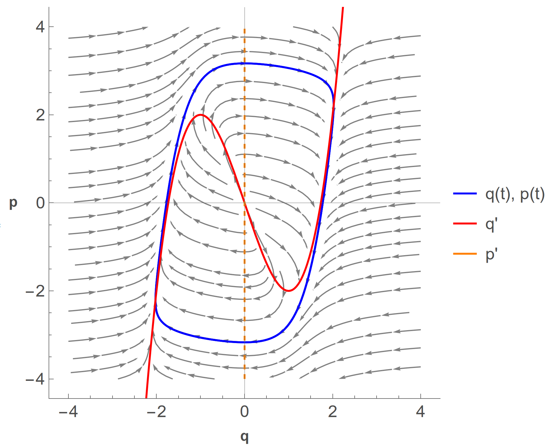
So I've been plotting phase portraits along with nullclines and phase flow for certain oscillators as follows:

tmax = 200; solution = NDSolve[{
   f''[t] + f[t] + f'[t]^{3} - 3 f'[t] == 0,
   f[0] == 3,
   f'[0] == 3
   },
  f, {t, 0, tmax}, MaxSteps -> 100000, AccuracyGoal -> 12, 
  PrecisionGoal -> 12]

splot = StreamPlot[{y - x^3 + 3 x, -x}, {x, -4, 4}, {y, -4, 4}, 
   StreamColorFunction -> {None}, StreamStyle -> {Gray}, Axes -> True,
    Frame -> {True, True, False, False}, 
   FrameLabel -> {Style["q", Bold, 12], Style["p", Bold, 12]}
   , RotateLabel -> False,
   PlotLegends -> 
    Placed[LineLegend[{Blue, Red, Orange}, {"q(t), p(t)", "q'", 
       "p'"}] , Right], LabelStyle -> {14, GrayLevel[0.3]}];
plot1 = ParametricPlot[
   Evaluate[{-f'[t], f[t]} /. solution], {t, 180, 200}, 
   PlotStyle -> {Blue}, PlotRange -> All];
nplot1 = Plot[{y = x^{3} - 3 x}, {x, -4, 4}, PlotStyle -> {Red}];
nplot2 = 
  ContourPlot[x == 0, {x, -4, 4}, {y, -4, 4}, 
   ContourStyle -> {Orange, Dashed}];
Show[splot, plot1, nplot1, nplot2]

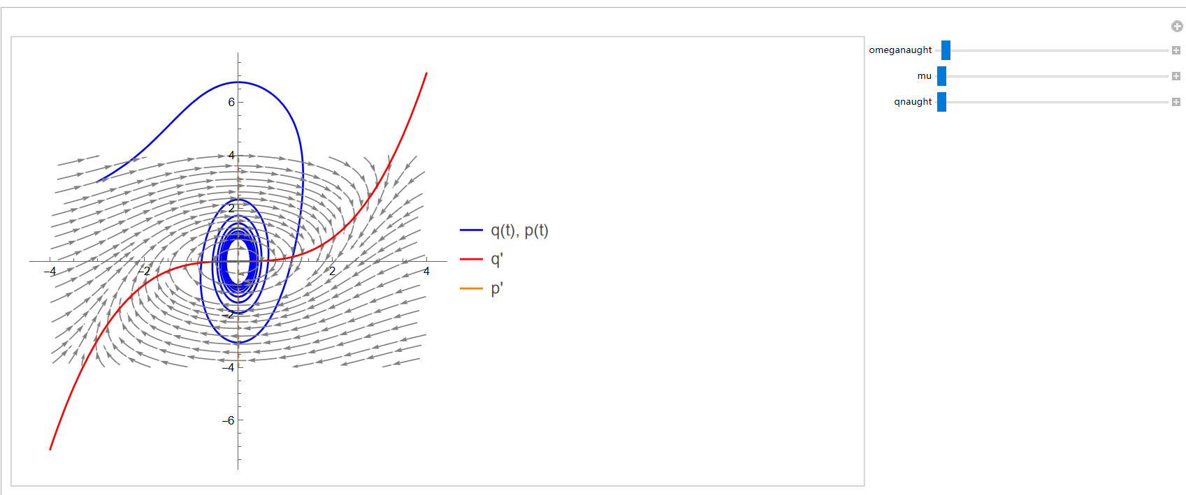
which gives: I'd like to create a similar plot which allows me to manipulate the parameters omeganaught, mu, and qnaught. I've tried the following code to no avail, and I'm not sure where to go from here.

sol = ParametricNDSolveValue[{
   p''[t] + omeganaught^{2}*p[t] + 
     mu*((1/(3*omeganaught))*p'[t]^{3} - qnaught^{2}*p'[t]) == 0,
   p[0] == 3,
   p'[0] == 3
   },
  {p}, {t, 0, 200}, {omeganaught, mu, qnaught}, MaxSteps -> 1000000, 
  AccuracyGoal -> 12, PrecisionGoal -> 12]

plot2 = Manipulate[
   ParametricPlot[
    Evaluate[
     {-p'[t], p[t]} & /@ sol[omeganaught, mu, qnaught]], {t, 0, 200},
    PlotStyle -> {Blue},
    PlotRange -> All],
   {{omeganaught, 0.1}, 0, 10}, {{mu, 0.1}, 0, 10}, {{qnaught, 0.1}, 
    0, 10}];

splot1 = StreamPlot[
   {omeganaught*y - mu*(((x^{3})/3) - qnaught^{2}*x), -omeganaught*
     x},
   {x, -4, 4}, {y, -4, 4},
   StreamColorFunction -> {None}, StreamStyle -> {Gray}, Axes -> True,
    Frame -> {True, True, False, False}, 
   FrameLabel -> {Style["q", Bold, 12], Style["p", Bold, 12]}
   , RotateLabel -> False,
   PlotLegends -> 
    Placed[LineLegend[{Blue, Red, Orange}, {"q(t), p(t)", "q'", 
       "p'"}] , Right], LabelStyle -> {14, GrayLevel[0.3]}];

nplot3 = Plot[
   {y = (mu/omeganaught)*(((x^{3})/3) - qnaught^{2}*x)}, {x, -4, 4}, 
   PlotStyle -> {Red}];

nplot4 = 
  ContourPlot[x == 0, {x, -4, 4}, {y, -4, 4}, 
   ContourStyle -> {Orange, Dashed}];

Show[splot1, plot2, nplot3, nplot4]

I end up with an error "could not combine the graphics objects in show". Even when I try just the ParametricPlot I end up with a blank plot.

I apologize for the long question.

Answer 1

• Using ParametricNDSolve and solve {p, p'} simultaneously.

• We need to replace x^{3} and qnaught^{2} by x^3 and qnaught^2.

Clear["Global`*"];
sol = ParametricNDSolve[{p''[t] + omeganaught^{2}*p[t] + 
      mu*((1/(3*omeganaught))*p'[t]^{3} - qnaught^{2}*p'[t]) == 0, 
    p[0] == 3, p'[0] == 3}, {p, p'}, {t, 0, 200}, {omeganaught, mu, 
    qnaught}, MaxSteps -> 1000000, AccuracyGoal -> 12, 
   PrecisionGoal -> 12];
Manipulate[
 {ParametricPlot[{-p'[omeganaught, mu, qnaught]@t, 
      p[omeganaught, mu, qnaught]@t} /. sol, {t, 0, 200}, 
    PlotStyle -> {Blue}, PlotRange -> All, 
    PerformanceGoal -> "Quality", AspectRatio -> 1],
   StreamPlot[{omeganaught*y - 
      mu*(((x^3)/3) + qnaught^2*x), -omeganaught*x}, {x, -4, 
     4}, {y, -4, 4}, StreamColorFunction -> {None}, 
    StreamStyle -> {Gray}, Axes -> True, 
    Frame -> {True, True, False, False}, 
    FrameLabel -> {Style["q", Bold, 12], Style["p", Bold, 12]}, 
    RotateLabel -> False, 
    PlotLegends -> 
     Placed[LineLegend[{Blue, Red, Orange}, {"q(t), p(t)", "q'", 
        "p'"}], Right], LabelStyle -> {14, GrayLevel[0.3]}],
   Plot[{y = (mu/omeganaught)*(((x^3)/3) - qnaught^2*x)}, {x, -4, 4}, 
    PlotStyle -> {Red}],
   ContourPlot[x == 0, {x, -4, 4}, {y, -4, 4}, 
    ContourStyle -> {Orange, Dashed}]} // Show, {{omeganaught, 0.3}, 
  0, 10}, {{mu, 0.1}, 0, 10}, {{qnaught, 0.1}, 0, 10}]