Generate a list of numbers based on histogram data

Question

Given the following histogram data: {{0, 1/10, 1/5, 3/10, 2/5, 1/2, 3/5, 7/10, 4/5, 9/10, 1}, {129, 57, 46, 42, 40, 40, 43, 45, 57, 129}}. That correspond to the following histogram plot:

Is there straightforward way to generate a list of numbers that adhere to this distribution?

Answer 1

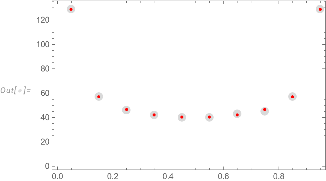
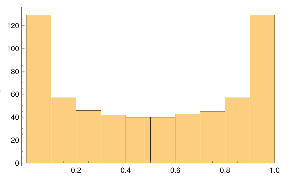
Because this histogram looks like it could have been generated by random samples from a beta distribution, one should attempt to see if a beta distribution might be a good fit. Then samples can be easily generated.

Here is how to find the maximum likelihood estimates of the parameters of a beta distribution given that you have histogram counts rather than the raw data:

h = {{0, 1/10, 1/5, 3/10, 2/5, 1/2, 3/5, 7/10, 4/5, 9/10, 1},
     {129, 57, 46, 42, 40, 40, 43, 45, 57, 129}};

(* Log of the likelihood *)
logL = Sum[h[[2, i]] Log[CDF[BetaDistribution[a, b], h[[1, i + 1]]] - 
      CDF[BetaDistribution[a, b], h[[1, i]]]],
  {i, 1, Length[h[[2]]]}];

(* Find maximum likelihood estimates of the beta distribution parameters *)
mle = FindMaximum[{logL, a > 0 && b > 0}, {{a, 0.5}, {b, 0.5}}]
(* {-1369.97, {a -> 0.500075, b -> 0.500075}} *)

(* Expected frequencies based on maximum likelihood estimates *)
freq = Total[h[[2]]] Table[
   CDF[BetaDistribution[a, b] /. mle[[2]], h[[1, i + 1]]] - 
    CDF[BetaDistribution[a, b] /. mle[[2]], h[[1, i]]], {i, 1, 
    Length[h[[2]]]}];

(* Plot histogram counts and expected counts given the maximum likelihood estimates *)
midpoints = (h[[1, 2 ;; Length[h[[1]]]]] + 
     h[[1, 1 ;; Length[h[[1]]] - 1]])/2;
ListPlot[{Transpose[{midpoints, h[[2]]}], 
  Transpose[{midpoints, freq}]}, 
 PlotStyle -> {{LightGray, PointSize[0.03]}, {Red, PointSize[0.01]}}, 
 Frame -> True]

If this is close enough fit, then generating random samples can be accomplished with

n = 20; (* Desired sample size *)
SeedRandom[12345];
data = RandomVariate[BetaDistribution[a, b] /. mle[[2]], n]
(* {0.119018, 0.768008, 0.189099, 0.982438, 0.542633, 0.357933, 0.63071, 
0.135144, 0.0504953, 0.984192, 0.839265, 0.0853941, 0.290643, 
0.672462, 0.98937, 0.769257, 0.753709, 0.833316, 0.452736, 0.997032} *)

Answer 2

Here is my sample code.

{bins, hist} = {{0, 1/10, 1/5, 3/10, 2/5, 1/2, 3/5, 7/10, 4/5, 9/10, 
1}, {129, 57, 46, 42, 40, 40, 43, 45, 57, 129}};

data = Flatten[RandomReal[#[[1]], #[[2]]] & /@ 
Transpose[{Partition[bins, 2, 1], hist}]]

The variable "data" contains what you want. If you want to randomize the order, then just

data = RandomSample[data]

will suffice.