Extended Comment rather than answer
TL;DR An implicit equation can be interesting for an analysis of the function's characteristics. There are some use cases where it might be better than using NDSolve but I do not know of many scenarios like that. For this particular implicit function, I did not find much that one could use. As such, the following text does not contain anything particularly interesting and is kind of an extended comment
The implicit solution given by DSolve can be useful theoretically or numerically but I would say mostly theoretically although I could be wrong.
Theoretically: An analysis of the implicit solution can provide crucial insights about a function. It can provide the domain in which it is defined, bounds, singularities and asymptotic behavior.
Moreover, an implicit definition involving integrals might have interesting change of variables and integrations by parts that might highlight details about the function. Finally, an implicit solution gives a more natural way to extend the function to the complex plane to study the types and numbers of singularities around the real line (which affects matters such as how easy it is to numerically integrate such a function in a given interval)
Numerically: It provides an alternative means to solve the equation, that is, the possibility to consider also FindRoot if NDSolve gave issues for the problem at hand. FindRoot could be faster if one only wants the endpoint of the integration and one has a good guess for this point either by looking at the graph or by prior analytical computations. If an entire interval is needed I would imagine that NDSolve would be faster unless there is an intermediate singularity in the way.
Consider then the example given.
First notice that the $\log(K[1])$ in the integral on the left hand side with the upper bound $\frac{y(x)}{x}$ and the $\log(x)$ on the right hand side shows us that this definition only applies to $x>0$ and $y(x)>0$. Hence, we will restrict the following discussion to this domain.
To get the function that defined the implicit equation one can do:
sol = DSolve[{y'[x] == 2*Log[y[x]/x], y[4] == 7}, y[x], x][[1]]

aux[y_, x_] = sol[[1]] - sol[[2]] /. y[x] -> y /. Integrate -> NIntegrate

f[y_?NumericQ, x_?NumericQ] := aux[y, x] // Activate;
Graphs
The implicit equation is then defined by f[y,x]=0. And one can find the curve y[x] by looking for the contour where f[y,x]=0 using ContourPlot.
ContourPlot[f[y, x], {x, 0, 20}, {y, 0, 12}, PlotLegends -> Automatic]

The self added 0 in the image annotation is visible when hovering over the curve in Mathematica. That curve represents the y[x] that one seeks.
Theoretical part: analysis of the implicit equation using insights from the graph
Notice that this curve is bounded in the upper left plane and y[x] goes to 0 both for x=0 and for some special x. To find that x analytically one can consider the behavior of the integral when the upper-bound goes to zero as the upper bound is $\frac{y(x)}{x}$. The behavior of the integral in special regions can be found sometimes with AsymptoticIntegrate. However, after waiting some time I did not receive an answer from Mathematica using AsymptoticIntegrate.
Instead we can use the implicit equation to find the coordinates of the maximum.
At the maximum, one has $y'(x_0)=0$. Using that within the original differential equation, we may deduce from $\log(\frac{y(x_0)}{x_0})=0$ that $y(x_0)=x_0$. Now the implicit equation part, one may use that in the implicit equation to obtain $\log(x_0)$ as a combination of integrals thereby allowing us to find an analytical formula for $x_0$ and $y(x_0)$. Not that much but in another example one could get nice asymptotics.
Numerical Part
As mentioned above one can find y[x] using NSolve with the implicit equation. I do not see any benefit of doing that in this case but for the sake of comparison with NDSolve I will.
Initialization:
yroot[1] = 0; iterations = 40;
xstart = 0.5; xend = 18.5;
xlist = Subdivide[xstart, xend, iterations];
follow the solution by continuity updating the guess with prior solutions:
Do[yroot[i + 1] = y /. FindRoot[f[y, xlist[[i + 1]]] == 0,
{y, yroot[i]}], {i, iterations}]
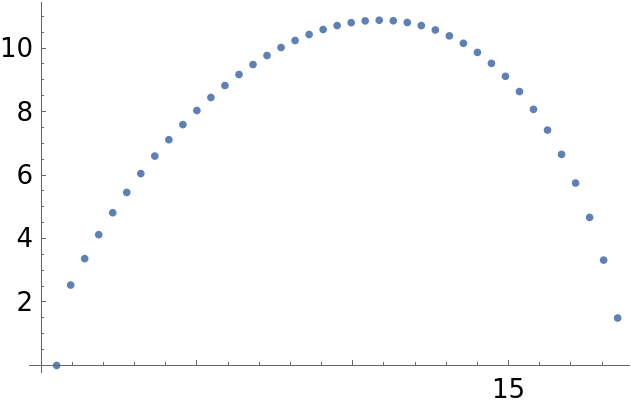
The graph:
Transpose[{xlist, yroot /@ Range[iterations + 1]}] // ListPlot

Comparison with NDSolve
Plot[Evaluate@NDSolveValue[{y'[x] == 2*Log[y[x]/x], y[4] == 7}, y[x], {x, 0, 18.5}], {x, 0, 18.5}]

Summary
In this case it is hard to find a theoretical or numerical benefit to the implicit solution provided but in general an implicit solution can be an opportunity to obtain more precise statements than the visual look of a graph.


