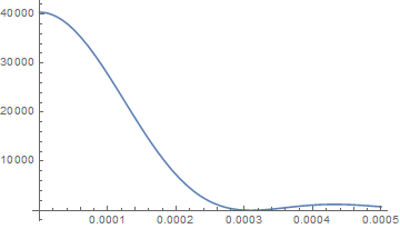
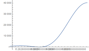
The issue with this integrand seems to be the highly oscillatory nature which makes it difficult to find the right step spacing. In the following I will give two methods to deal with the small step sizes.
The integrand:
g[t_] = Cos[2022*t]*Sin[10050*t]*Sin[10251*t]/Sin[50*t]/Sin[51*t]
First method: integration using NDSolve
One possibility is to use the adaptive methods of NDSolve to find the right step sizes:
Edit: As recommended in the comments, I changed the starting point from 10^(-12) to $MachineEpsilon/2
AbsoluteTiming[
NDSolveValue[{v'[t] == g[t], v[$MachineEpsilon/2] == 0},
v[2 Pi], {t, $MachineEpsilon/2, 2 Pi}]/(6*Pi) - 1]
output: (*{0.391597, -2.92904*10^-6}*)
If we need more precision we can adjust the options of NDSolve, for example :
AbsoluteTiming[
NDSolveValue[{v'[t] == g[t], v[$MachineEpsilon/2] == 0},
v[2 Pi], {t, $MachineEpsilon/2, 2 Pi}, PrecisionGoal -> 10,
AccuracyGoal -> 10, Method -> "ExplicitRungeKutta"]/(6*Pi) - 1] (* relative error *)
output: (*{0.438849, 1.79297*10^-10}*)
Second method: summing over sub-intervals specified by the zeroes of the function.
A more manual approach is to consider a partition of the interval defined by the zeroes of the function.
Specifically, for x[r] the r'th zero of the integrand, we consider the following partition of the original interval Interval[0,2*Pi]=IntervalUnion[Interval[x[0],x[1]],Interval[x[1],x[2]],....] (this is just a representation not part of the code)
Find the zeroes:
Using Solve or SolveValues takes a lot of time. As such, Reduce is used instead as it is roughly seven times faster in this case :
a = Reduce[Cos[2022*t]*Sin[10050*t]*Sin[10251*t] == 0 && 0 <= t <= 2*Pi, t];
However, the output format is a mixture of equalities and inequalities for auxiliary constants. The code below extracts and constructs numerical zeroes from the output of Reduce:
zeroes = (List @@ a[[;; -5, 2]])~Join~
  DeleteDuplicates[Apply[Join, (#[[3, 2]] /. C[1] -> Range[0, #[[2, 5]]] &) /@ a[[-4 ;; -1]] ]]
Next, we use Gauss-Legendre points in each sub-interval. The most (computer) efficient way might be to use
NIntegrate`GaussKronrodRuleData[points,precision]
as used in the documentation on integration rules and then rescale the points according to the sub-intervals. However, for brevity and convenience, we will use GaussianQuadratureWeights from the NumericalDifferentialEquationAnalysis` package:
Needs["NumericalDifferentialEquationAnalysis`"]

points = (GaussianQuadratureWeights[21, ##] &) @@@
Partition[Sort@zeroes, 2, 1];

pointsf = SortBy[Join @@ points, First];

Total[pointsf[[All, 2]]*g[pointsf[[All, 1]]]]/(6*Pi) -
1 // AbsoluteTiming (* relative error *)
output: (* {0.151416, 8.65974*10^-13} *)
One should also consider the time used to obtain the zeroes but if the integral has to be used for a range of frequencies, using Reduce symbolically would be a one time cost.


MinRecursion -> 8, Method -> {"GaussKronrodRule", "Points" -> 21}. $\endgroup$NIntegrate[ Cos[2022*t]*Sin[10050*t]*Sin[10251*t]/Sin[50*t]/Sin[51*t], {t, 0, 2*Pi}, Method -> {"LevinRule", "Kernel" -> Cos[2022*t]}, MaxRecursion -> 8]results in8.75152which is far away from the right one. $\endgroup$