Find min and max indices of highest and lowest elements in sorted list

Question

I have a list of integers of the form

Nmax = 17000;
list1 = Join[Table[0, 560], 
   FoldList[Min[Nmax, Plus[#1, #2]] &, 0, 
    RandomChoice[{0, 1, 2}, Nmax + 8100]]];

(the numbers are kind of arbitrary--I just wanted to construct a list with many 0's at first, a sorted middle and then a large plateau above some fixed value, here Nmax). My question is the following: I would like to find the indices corresponding to the last 0 and the first Nmax. Or, equivalently, I want to find the indices between which the list is not 0 or Nmax, which corresponds to the maximum index whose element is 0 and the minimum element whose value is Nmax. This can be accomplished pretty simply with the following code:

{lower, upper} = {1 + (Last@Position[list1, 0])[[1]], -1 + (First@
      Position[list1, Nmax])[[1]]}
list2=list1[[lower;;upper]]

However, I would like to run this code on many thousands of different lists, and the above code seems to take longer than necessary to find lower and upper, since Position makes no use of the fact that list1 is sorted. Is there a way to get these two indices in a more efficient way?

Answer 1

OP may want to use binary search. There are many posts here on Mathematica SE relating to binary search, including this which also contains compiled code. See also this.

Code. To find the highest index with entry zero, one can use

(* list must be a sorted list of integers >= 0 *)
maxindex0[list_]:=Module[{l=0,r=Length[list]+1},
  While[l<r-1,With[{m=Floor[(l+r)/2]},
    If[list[[m]]==0,l=m,r=m]]];
l];

Example.

SeedRandom[1];
example=Map[Max[0,#]&,Sort[RandomInteger[{-100,1000},1000000]]];

Then

RepeatedTiming[(Last@Position[example,0])[[1]]]
{0.0671354, 92178}

RepeatedTiming[maxindex0[example]]
{0.0000641912, 92178}

So OPs code takes about 50 milliseconds, maxindex0 takes about 0.05 milliseconds.

Answer 2

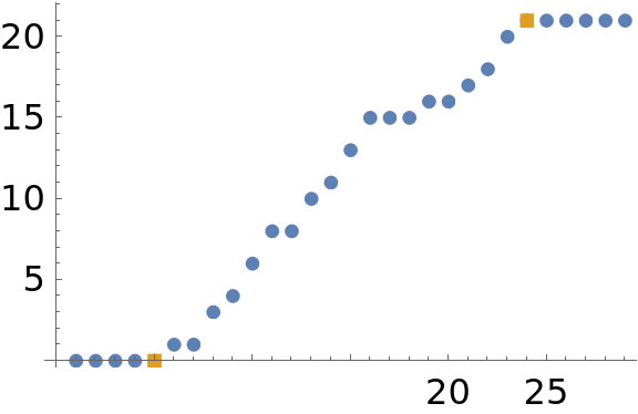
Graphical explanation of what I understood OP's wants:

list1= {0, 0, 0, 0, 0, 1, 1, 3, 4, 6, 8, 8, 10, 11, 13, 15, 15, 15, 16, 16, \
     17, 18, 20, 21, 21, 21, 21, 21, 21}

The list above was generated using OP's code.

Plotting the list:

ListPlot[{list1, {{5, 0}, {24, Nmax}}}, 
 PlotMarkers -> {Automatic, 0.04}, ImageSize -> Small]

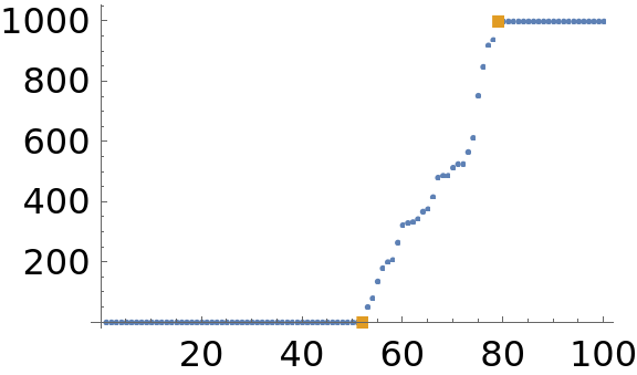
With a list that has more points:

SeedRandom[42];
max = 1000;
size = 100;
test = Clip[
   Sort@RandomInteger[{-Floor[2*max], Floor[2*max]}, size], {0, 
    max}];

As I understand, the abscissas of the two squares are the values requested by OP. That is, the position of the last 0 of the initial plateau and the position of the first point in the last plateau (the first Nmax using OP's notation).

---

If speed is not much of a concern:

The solution proposed by @Syed is in my opinion rather convenient. Here is another possibility:

  last0=LengthWhile[list, # == 0 &]

  firstNmax= First@FirstPosition[list, Nmax]

---

If you want the quickest method in the generic case :

See @293787's answer.

---

If the length of one plateau is relatively small (smaller than Log2[Length[list]])

and so your case is not generic, then the following can be of use.

TL;DR: If the length of the first plateau is small use LengthWhile. If the length of the last plateau is small, then reverse the order of the elements in the list and use LengthWhile

As you would like something that is fast, the Position function might not be the best option as it will search the entire list. That is unneeded in your case as your lists are sorted. For example, it is clear that, starting from the first element of the list list[[1]], it is no longer necessary to scan the list after the first encountered non zero element.

Test list :

SeedRandom[42];
max = 1000;
size = 100;
ratio = 1;
test = Clip[
   Sort@RandomInteger[{-Floor[2*max], Floor[2*max*ratio]}, size], {0, 
    max}];

Changing "ratio" you may change the ratio between the lengths of the first and last plateaus.

To check the validity of the codes below you may add indices to the test list and maybe decrease the size :

{test,Range[Length[test]]}//Transpose 

{{test[[1]],1},{test[[3]],2},...}

The fastest method will depend on the lengths of the plateaus. If we subdivide the previous plot in 3 parts:

Big Plateau 1 (BP1), Rocky Hill (RH), Big Plateau 2 (BP2)

Then, for example, it could be advantageous to scan the list backwards if Length[BP2] is a lot smaller than Length[BP1] or Length[RH]. Specifically, you have 3 scenarios:

1. If : you already know beforehand that Length[BP1]/Length[list] is very small (smaller than Log2[Length[list]])

   Then : you can obtain the last 0 efficiently with

       last0=LengthWhile[list, # == 0 &]
   

   (* Remark : using FirstPosition[list, _?(#!=0 &)] or Position[list1, 0][[-1, 1]] takes a lot more time in this case)

2. If : you already know beforehand that Length[BP2]/Length[list] is very small (smaller than Log2[Length[list]]) Then: you can obtain the first Nmax efficiently with

   listLength=Length[list1]

   firstNmax = listLength - LengthWhile[list1[[-1 ;; 1 ;; -1]], # == Nmax &]+1

3. Else: In the the generic case, a C-Compiled version of the method provided by @user293787 will likely be optimal.

---

BenchMarking the methods proposed so far:

The following benchmarks are for the generic case where the length of both plateaus are large. If one of the plateaus is relatively tiny use LengthWhile (see discussion of the previous section).

For a more complete comparison I will include a C compiled function (you may remove CompilationTarget -> "C" if you do not have a Compiler with Mathematica). The function below does a forward scan and works with an integer list. As discussed above, if the last plateau is shorter than the first plateau it can be advantageous to do a backward scan instead :

edgeplateau = Compile[{{list, _Integer, 1}, {Nmax, _Integer}},
  Module[{index1 = 0, index2 = 0, a = 0}, 
   While[a == 0, index1 += 1; a = list[[index1]]];
   index2 = index1; 
   While[a < Nmax, index2 += 1; a = list[[index2]]]; {index1-1, 
    index2}], CompilationTarget -> "C"]

output of edgeplateau: {last 0, first Nmax}

Test List:

Nmax = 200000;
list1 = Join[Table[0, 3000000], 
      FoldList[Min[Nmax, Plus[#1, #2]] &, 0, 
        RandomChoice[{0, 1, 2}, Nmax + 3000000]]];

Properties of test list: the length of the first plateau is roughly the same as the last plateau and rocky hill climb between the two is relatively quite thin (like a cliff).

Methods for finding the last 0:

AbsoluteTiming[last0=First@FirstPosition[list1, _?(#!=0 &)]-1;]

{0.799981, Null}

*Below: Method by @UlrichNeumann*

AbsoluteTiming[last0 = Position[list1, 0][[-1, 1]];]

{0.631989, Null}

AbsoluteTiming[LengthWhile[list1, # == 0 &];]

{0.588371, Null}

*Below: maxindex0 is defined in @user293787's answer, see also links *

AbsoluteTiming[maxindex0[list1];]

{0.000104, Null}


*C compiled maxindex0 with where the list elements are expected to be integers*

 {0.000043, Null}

Methods for finding the first Nmax:

Position[list1, Nmax][[1, 1]]; // AbsoluteTiming

{0.636139, Null}

FirstPosition[list1, Nmax]; // AbsoluteTiming

{0.164197, Null}


last0 + FirstPosition[list1[[last0 ;;]], Nmax] - 1; // AbsoluteTiming

{0.106541, Null}

LengthWhile[list1, # != Nmax &] + 1; // AbsoluteTiming

{0.782357, Null}


last0 + LengthWhile[list1[[last0 ;;]], # != Nmax &]; // AbsoluteTiming

 {0.055123, Null}

An equivalent of maxindex0 to find the first Nmax will have similar speed when compared to the timing of maxindex0

Methods for finding both the last 0 and the first Nmax:

* @Syed's answer *

{Last@First@#, First@Last@#} &@PositionIndex[list1] // AbsoluteTiming

{0.148351, Null}

*compiled edgeplateau*

AbsoluteTiming[edgeplateau[list1, Nmax];]

{0.026304, Null}


*uncompiled edge plateau*

{1.77486, Null}

Answer 3

What about

last0 = Position[list1, 0][[-1, 1]] (* 562*)
firstN = Position[list1, Nmax][[1, 1]](*17626*)

Answer 4

SeedRandom[1];
Nmax = 17000;
list1 = Join[Table[0, 560], 
   FoldList[Min[Nmax, Plus[#1, #2]] &, 0, 
    RandomChoice[{0, 1, 2}, Nmax + 8100]]];


{Last@First@#, First@Last@#} &@PositionIndex[list1]

{561, 17629}