Edit: For problems with few roots in the domain of parameters considered (or low dimensional simple manifolds) and when function evaluation is not costly, it might be better to skip the long discussion below and use the visual method by @Akku14 and the numerical method by @AlexTrounev.
In the following I will discuss general methods with simple examples and in the end I will discuss a possible solution to the original problem
The question does not seem specific to mathematica and is more of a question on numerical methods. Hence, you might get a broader range of answers by looking at other parts of stack exchange that deal with numerical methods. Not sure which one, maybe the stack exchange on mathematics as there might be applied mathematicians there.
I actually worked on a similar situation and I am planning on publishing a paper that will use the method that I explain below. The solution was inspired from references I read on the homotopy analysis method (you do not need to know it to understand the following) although the explanation you will find on Wikipedia about this method might not give you the broad idea of the method.
Let $x$ be the solution of a system of potentially non linear equations denoted as ${\cal N}$ with parameters $\theta=(\theta_1,\theta_2,...)$:
${\cal N}[x,\theta]=0$
$x$ could have many components but in the examples of this first part we will focus on a 1-dimensional problem. The original problem is 2-dimensional and I will give an answer for that problem in the second part.
Example
(*Below ${\cal N}$=eq, g=$x$ , $\theta$={ll,r} *)
eq[g_,l_,r_]=Cos[r*g]+ll*Sin[g]; eq[g,ll,r]==0
According to the implicit function theorem $x$ is a function of $\theta$. We will take the hypothesis that $x$ is a smooth function of $\theta$.
First, for all the methods below you need a good starting point. Sometimes $\theta=0$ or $\theta=1$ will suffice and maybe sometimes you should use RandomReal. If there is a limit of the parameters where the problem becomes simple then you might want to consider obtaining some analytical results using perturbation theory in that limit to get a good starting point. It is possible that the limit itself plus maybe some random noise can be enough to get a good starting point for FindRoot when the parameters are close to that limit.
Example:
Solve[eq[g,1,1],g] gives all solutions one being -Pi/4. ll=1 and r=1 will be our starting point.
The methods:
By continuity (robust and precise but slow)
Consider a starting point $\theta=\theta^{(0)}$ and a grid of (multi-dimensional) points $\theta^{(i)}$ with $\theta^{(i)}-\theta^{(i+1)}$ small. Then, you can a make a program that operates as a for loop that finds the solution for $\theta^{(i)}$ with FindRoot and that uses that solution as an initial condition for the point $\theta^{(i+1)}$.
Example:
(* intialization *)
g0=-Pi/4;
ll=1;
groot[1]=g0;iterations=10;
rstart=1.;rend=5.;
rlist=Subdivide[rstart,rend,iterations];
(* iteratively obtaining roots *)
Do[

 groot[i+1]=g/.FindRoot[eq[g,ll,rlist[[i+1]]]==0,{g,groot[i]}]

 ,{i,iterations}]
(* Verifying the roots *)
MapThread[eq[#1,ll,#2] &,{groot/@Range[iterations+1],rlist}]
output:
(* {1.1102210^-16, 0., 0., -5.5511210^-17, 0.,
5.5511210^-17, -1.1213310^-14, -4.3298710^-15, -1.8318710^-15,
-7.2164510^-16, -2.7755610^-16} *)
By differentiability (quick)
In this method you turn the problem to a differential equation by taking a derivative of the equation and then using NDSolve. I like this method because the adaptive methods of NDSolve finds the step size for you and changes it automatically if it thinks it needs a smaller step size.Also in principle this should allow bigger step sizes as the the guess for the next step uses both the value and the slope of the previous step whereas the continuity method only looks at the previous value. However, in my experience, I have struggled to get bigger step sizes then what NDSolve does automatically. I also suggest checking sometimes if the results you find with this method do solve the non linear equation you have. This might also be true with the method above.
As mentioned before the solution $x$ is actually a function of the parameters $\theta$ of the equation. Hence the equation can be written more explicitly as :
${\cal N}[x(\theta),\theta]=0$
Taking the derivative of the equation above with respect to one of the parameters in $\theta$ which we will choose to be $\theta_1$, we obtain a differential equation:
$\partial_{\theta_1} x(\theta)\partial_x{\cal N}[x(\theta),\theta]+\partial_{\theta_1}{\cal N}[x(\theta),\theta]=0$
Example:
dreq[l_,r_]=D[eq[g,l,r]/.g->g[r],r]
Because of the coefficient $\partial_x{\cal N}[x(\theta),\theta]$ that multiplies $\partial_{\theta_1} x(\theta)$, in my experience, the above differential equation is often stiff and if you try to solve it with NDSolve you will receive an error (this does not happen with the example provided). However, if I remember correctly Mathematica also suggests an option that allows it to work with stiff equations. I do not remember the name of the option but if you try this and do not see the suggestion by Mathematica then please write a comment below and I will search my files for the option.
Once that option is included, you can solve the differential equation with a starting point $(\theta_1^{(\textrm{start})},\theta_2^{(0)},...)$, an end point $(\theta_1^{(\textrm{end})},\theta_2^{(0)},...)$ and an initial condition for $x$ at $\theta_1^{(\textrm{start})}$ which will give you $x(\theta)$ in that range.
Example:
rstart=1;
rend=5;
g0=-Pi/4
ll=1;
gsol=NDSolveValue[{dreq[ll,r]==0,g[rstart]==g0},g,{r,rstart,rend}]
Testing the accuracy:
Plot[Abs[eq[gsol[r],ll,r]],{r,rstart,rend}]
output: 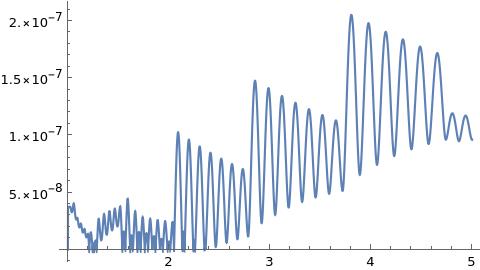
The precision is good but not as precise as with FindRoot, this is maybe related to the automatic values in PrecisionGoal and AccuracyGoal in NDSolve. You can try to choose your own precision if you want.
In your problem this would be one line in the cube of parameters you have and you can consider the cube of points as a cube of lines in the different parameters. You can decide how you want to space the lines.
The initial condition for $\theta_1=\theta_1^{(\textrm{start})}$ can be obtained using FindRoot or analytical results in some limit of the parameters. If I remember correctly this method works only if you have a good initial condition.
If the equation has a singularity in the domain you are searching (not necessarily the function itself it could be a derivative of the function) then the adaptive methods of NDSolve will choose smaller and smaller steps until the integration is not possible. A singularity maybe means that the program is at the boundary of the manifold defined by the set of roots of the equations.
I like to see the steps that NDSolve is taking in real time when using this differential equation method. If you are interested I can search my notebook for how I did it but it probably involves StepMonitor in NDSolve and using the function Dynamic to plot the points in real time (for my problem plotting in real time did not add much extra time but for your problem it might as it is possibly simpler).
Errors can accumulate over large domains when using the NDSolve method, so you might want to check if the solution obtained by NDSolve is really a root of the initial non linear equation. Also, you might want to polish the results (increase accuracy) by using FindRoot with the result from NDSolve as an initial condition.
Edit (! These are suggestions that I have not tried really): One could also consider maybe by piecewise analyticity using a multi-dimensional Taylor-expansion in the parameters restricted perhaps to sub-domains of the original problem. Another possibility might be by simplicity using regularized neural networks that are trained on some examples. This method is by simplicity because regularized neural networks seem to have a bias towards simple functions and so if the shape of the manifold defined by the zeroes of the equations is simple, then a neural network might be a good option in some cases (maybe high dimensional ones I am not sure).
The original problem
Edit: I had modified the $\gamma$ function in an experiment and I might have not put the factors back correctly or something because after copy pasting your function again I got new results.
The main issues in applyting the method using differentiability is the Abs and Im in the function.
I removed all the Abs and you can check a posteriori whether the signs should be different.
Concerning the Im, taking a derivative you will get an expression with Im'[...].Mathematica's derivative seems to handle cases with Im badly so I defined a derivative for this problem (I took the minimal amount of properties needed for this problem, this derivative might not generalize well to other problems):
deri[a_+b_,r_]:=deri[a,r]+deri[b,r];
deri[a_,r_] /; FreeQ[a,r]:= 0
deri[a_*b_,r_] /; FreeQ[a,r]:= a*deri[b,r]
deri[w*h_,w]:=h+deri[h,w]
deri[Im[b_],r_]:=Im[D[b,r]]
I define also rules for Im so that it implements basic properties:
imrule={Im[a_ + b_] -> Im[a] + Im[b], Im[bta^m_.*y_] -> bta^m*Im[y], Im[w*y_] -> w*Im[y]}
setting up the equations from the original problem (I removed the Abs !!) :
eq1[d_, mu1_, bta_, w_, Ex_]=dlta[d, mu1, bta, w, Ex]-d//Simplify;
eq2[d_, mu1_, bta_, w_, Ex_,mu0_]=nn1[d, mu1, bta, w, Ex]+ mu1 - mu0 //Simplify;
eqlist[d_, mu1_, bta_, w_, Ex_,mu0_]={eq1[d, mu1, bta, w, Ex],eq2[d, mu1, bta, w, Ex, mu0]};
(* derivative in the direction of w *)
dweqlist[bta_, w_, Ex_, mu0_]=deri[#, w] & /@ eqlist[d[w], mu1[w], bta, w, Ex, mu0] /.imrule /.deri->D //Simplify;
(* intialization *)
btai=RandomReal[{0.01,5}];
Exi=RandomReal[{0.5,5}];
wi=RandomReal[{0,5}];
mu0i=RandomReal[{-5,5}];
parameter values: {btai, wi, Exi, mu0i}={2.65194, 1.39173, 4.91738, 4.48104}
{mu1i,di}={mu1,d}/.FindRoot[eqlist[d, mu1, btai, wi, Exi, mu0i],{{mu1,1},{d,3}}]
output: {1.09501, 1.33762}
Notice that d is non zero although it might seem that there only roots with d=0 (* Please check this as I might have missed a term while copy-pasting or something*)
To check this you can use the graphical method by @Akku14:
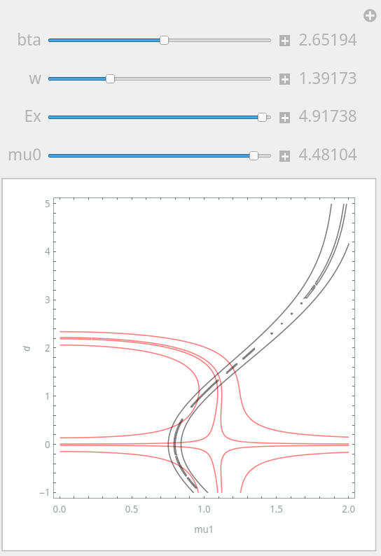
You can have a different view by plotting instead equation_1^2+equation_2^2 :
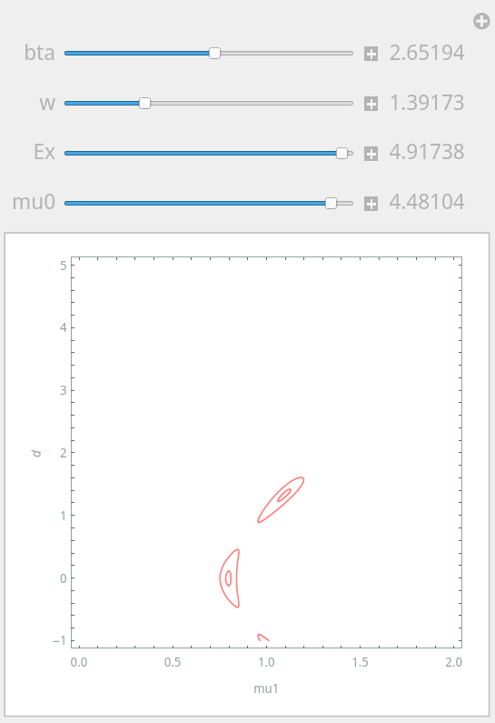
The roots are encircled by the red contours
(* obtaining d and mu1 for w belonging to the interval [wi, 5] *)
(Edit: I think the error I got about complex values was because of an experiment I did and I forgot to re-initialize the d[w] and mu1[w] with FindRoot)
{dsol,mu1sol}=NDSolveValue[Thread[dweqlist[btai, w, Exi, mu0i]==0]~Join~    {mu1[wi]==mu1i,d[wi]==di},
{d,mu1},{w,wi,5}]
The solver shows that it is unable to integrate pass w=2.118... and for a good reason as we will see.
(* Checking that the code works *)
Plot[eqlist[dsol[w], mu1sol[w], btai, w, Exi, mu0i],{w,wi,2.11}] (*{equation_1,equation_2}*)
output: 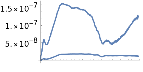
Let's see why the NDSolver had trouble pass w=w_c$\simeq 2.12$ :
Plot[{dsol[w], mu1sol[w]}, {w, wi, 2.11}, PlotLabels -> Automatic]
output: 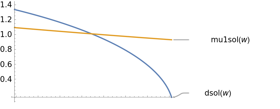
The function d goes to 0 in a singular manner that looks like sqrt if I had to guess. I show a contour plot near w_c below (I lowered the contour values to have a more detailed view):
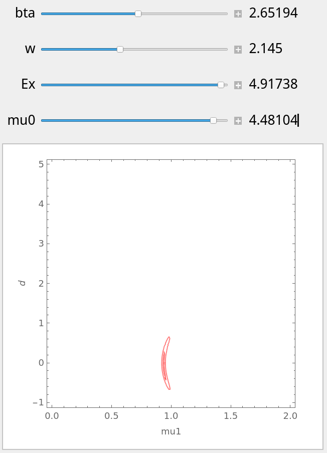
For w> w_c there is one root and for w<w_c there are three for the above chosen parameters. This is probably a pitchfork bifurcation similar to the mean-field equation of the Ising model (easy axis magnetism).
If there are physics behind these equations w=w_c might be the onset of new physics in the model (If the discussion above is not due to the fact that I omitted the Abs function)
PS: If there are physics behind those equations I am curious as to what they are as I am not used to seeing a Gamma function in the wild in physics. Otto Hölder's theorem says that the Gamma function is a hypertranscendental function (or a transcendentally transcendental function) and so it satisfies no algebraic differential equation whose coefficients are rational functions (and algebraic initial conditions). As most physics problems seem to be linked to differential equations in this category, it felt like I would never see this function in a physics problem (outside of string theory).


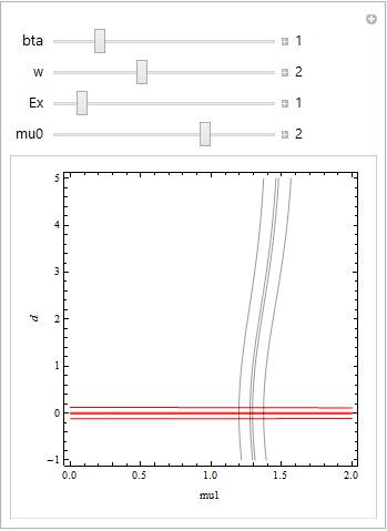
d==0, but probably you are not interested in them? You did not specify the range ofEx? Perhaps you can provide a concrete set of values for the arguments whereFindRootfails? SinceFindRootuses a Newton method by default, I would remove unnecessaryAbs, for example your first question has the form $||a|-|b|| = 0$ which can be written (assuming $a,b$ are real) in the form $a=b$ or $a=-b$ or $a^2 = b^2$. $\endgroup$