Algebraically, elip is easy to analyze and much easier if the coefficients are exact than floating-point numbers (easier for Mma, that is):
elipRat = Rationalize[Rationalize@elip, 0];
reg[t_] = ImplicitRegion[Log[1/2] == elipRat, {y, x}];
Show[
 Module[{color = 0},
  HighlightMesh[
     DiscretizeRegion@reg[#],
     {Style[0, None], Style[1, ColorData[97][++color]]}
     ] & /@ Rationalize@{1796.66, 2032.74, 2299.85}
  ],
 Frame -> True, FrameLabel -> Last@reg[t],
 AspectRatio -> 1
 ]
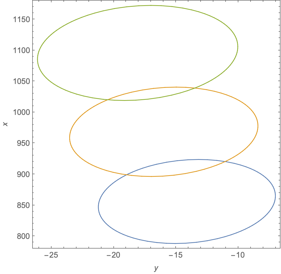
Switch {y, x} to {x, y} if you want the orientation to be in school-traditional order.
If you want to use features of ContourPlot, then the following shows where the plot should be focused:
N@RegionBounds@reg[#] & /@ Rationalize@{1796.66, 2032.74, 2299.85}
(*
{{{-21.2367, -7.01153}, {788.18,  923.789}},
 {{-23.5454, -8.41455}, {896.339, 1040.58}},
 {{-26.127,  -10.0327}, {1019.01, 1172.43}}}
*)
If you want to programmatically determine the range for ContourPlot with approximately optimal (minimal) sampling:
bnds = N@RegionBounds@reg[#] & /@  (* use reg[t] above *)
   Rationalize@{1796.66, 2032.74, 2299.85};
ctr = Mean@*Flatten /@ Transpose@bnds; (* center of sampling *)
{dy, dx} = (* min. diam. scaled by number < 1/Sqrt[2] *)
  Min /@ Map[Differences, Transpose@bnds, {2}]/GoldenRatio;
{yrange, xrange} = MinMax /@ Transpose@bnds; (* bounding ranges *)
yrange = {-150, 100}; xrange = {0, 4500}; (* desired ranges if different *)
{ny, nx} = Ceiling[Abs@({yrange, xrange} - ctrs[[All, 2]])/{dy, dx}];

ContourPlot[
 Evaluate@ (* makes three equations *)
  Thread[Log[0.5] == (elip /. t -> {1796.66, 2032.74, 2299.85})],
 (* align initial sampling grid on ctr *)
 {y, ctr[[1]] - First@ny*dy, ctr[[1]] + Last@ny*dy},
 {x, ctr[[2]] - First@nx*dx, ctr[[2]] + Last@nx*dx},
 (* adjust PlotPoints to {dy, dx} via {ny, nx} *)
 PlotPoints -> (Max[# + 1, 15] & /@ Total /@ {ny, nx})]
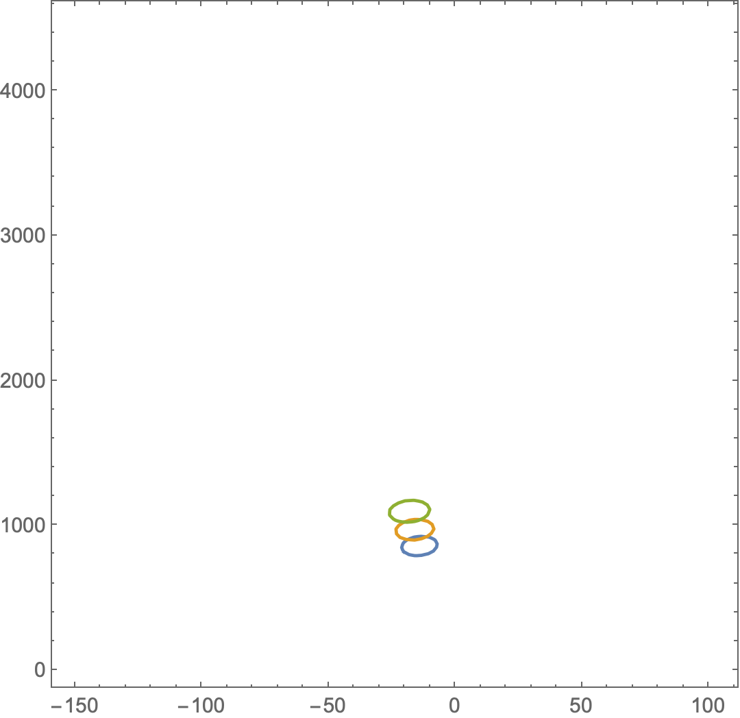
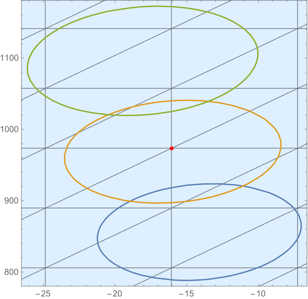
The following shows the initial sample mesh in the area around the ellipses. The important thing is to get at least one point inside each ellipse. I picked GoldenRatio for a safety factor (exceeds Sqrt[2]). Dividing by Sqrt[2] is on the boundary of optimal if the axes of the ellipses are parallel to the coordinate axes, which is not quite the case here. I didn't worry about the general case. The requirement is that any dy by dx rectangle should have at least one vertex in each ellipse. It works here. Clearly, extreme cases such as an ellipse that is nearly an oblique line segment may be extremely hard to deal with using ContourPlot.
I bumped up MaxRecursion to make the ellipses look pretty. The small ones above are jagged. In this case, the large MaxRecursion leads to refinement only in the neighborhood of the ellipses. It does not lead to the explosion of meshing one often gets and is quite quick in this case.
Show[
 ContourPlot[1,  (* initial sample mesh *)
  {y, ctr[[1]] - First@ny*dy, ctr[[1]] + Last@ny*dy}, {x,
   ctr[[2]] - First@nx*dx, ctr[[2]] + Last@nx*dx},
  PlotPoints -> (Max[# + 1, 15] & /@ Total /@ {ny, nx}),
  ColorFunction -> (LightBlue &),
  Mesh -> All, MaxRecursion -> 0],
 ContourPlot[    (* ellipses from above *)
  Evaluate@
   Thread[Log[0.5] == (elip /. t -> {1796.66, 2032.74, 2299.85})],
  {y, ctr[[1]] - First@ny*dy, ctr[[1]] + Last@ny*dy}, {x,
   ctr[[2]] - First@nx*dx, ctr[[2]] + Last@nx*dx},
  PlotPoints -> (Max[# + 1, 15] & /@ Total /@ {ny, nx}),
  MaxRecursion -> 5],
 Graphics[{Red, PointSize@Medium, Point@ctr}],
 PlotRange -> MinMax /@ Transpose@bnds
 ]

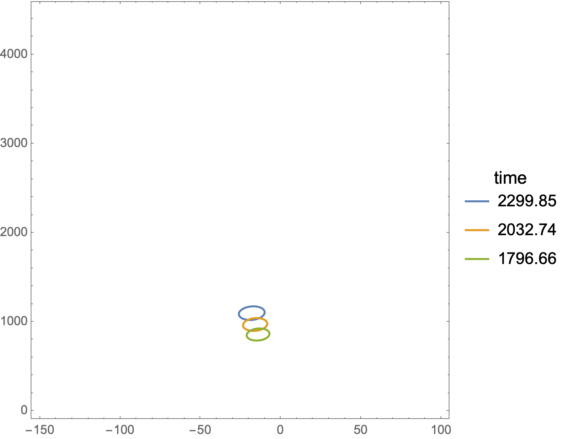


PlotPoints->100. $\endgroup$ContourPlotcan have trouble. An alternative would be aParametricPlot, but then you have to construct a parametrization first. $\endgroup$