Derivation of the Heston model from first principles using ItoProcess[ ]
It's pleasantly surprising that something as subtle and useful as the Heston PDE can be easily derived via ItoProcess, once a few hurdles are overcome along the way. It's useful because, although the std Heston derivation is retold intuitively and in detail by Wilmott, by Shaw, by Gatheral, and many others, once you have coded the basic derivation machinery in Mathematica you can use it safely and robustly to do derivations of your own proprietary PDE models with, say, "stochastic-local" volatility. And even before you start the PDE derivation you can do some very powerful explorations of the system of SDEs by, say, using the ItoProcess directly in the calculation option prices via monte-carlo, or by exploring symbolic correlation formulae of the components. And then once the derivation is complete, the resulting PDE can be used directly in NDSolve[ ] to calculate prices via, say, finite-difference or method-of-lines methods, or the PDE can be (after reformatting) pasted directly into a tool like SciFinance's SciPDE.
Initial reference: http://www.wolfram.com/mathematica/new-in-9/time-series-and-stochastic-differential-equations/heston-model.html (note that, as-at this post, it uses the v9.0 version of ItoProcess, and therefore the graphics at that URL are subtly incorrect due to the correlation matrix bug).
But first let me take this opportunity to acknowledge Mark Fisher. Before ItoProcess[ ], for many years I used his Mathematica package which can be found these days at http://www.markfisher.net/~mefisher/mma/ItosLemma.m. In some ways Mark's package is still preferable to ItoProcess[ ] because it allows you to work with correlated wieners whereas ItoProcess[ ], when it can, reduces the system of equations down to orthogonal processes. That causes some initial discomfort when you first try and match some canonical examples, say Wilmott or Shaw or Gatheral. Enough waffle…
Following the authors noted above, we start the derivation by defining the ItoProcess for two correlated Wieners. Note that this applies the function defined in my earlier post, ItoProcessDougs[ ], which fixes a bug in the built-in ItoProcess for correlated processes...
cW[ρ_] := ItoProcessDougs[{{0, 0}, IdentityMatrix2}, {{w1, w2}, {0, 0}}, t,
  {{1,ρ}, {ρ, 1}}];
cWproc = cW[ρ]

Correlation[cWproc1, 1, 2]
;

Out := ItoProcess[{{0, 0}, {{1, 0}, {ρ, Sqrt[1 -ρ^2]}},
  {w1[t], w2[t]}}, {{w1, w2}, {0, 0}}, {t, 0}]
ρ
Define the Heston model by SDEs driven by the correlated 2D Wiener process:
hm = ItoProcess[{
ds[t] == (μ - q) s[t]dt + Sqrt[V[t]] s[t]dws[t],

  dV[t] ==κ (θ - V[t])dt +ξ Sqrt[V[t]]dwν[t]},

  {s[t], V[t]}, {{s, V}, {s0, V0}}, t,
  {ws, wν}[Distributed] cW[ρ]]

ToSDEs[hm, {t, {ws, W}}](*where ws and W are uncorrelated Wieners*)


Out := ItoProcess[{{-q s[t] +μ s[t],θκ -κ V[t]},
  {{s[t] Sqrt[V[t]], 0}, {ξρ Sqrt[V[t]],ξ Sqrt[1 -ρ^2] Sqrt[V[t]]}},
  {s[t], V[t]}}, {{s, V}, {s0, V0}}, {t, 0}]


{dt (-q s[t] +μ s[t]) +dws[t] s[t] Sqrt[V[t]],
  ξ Sqrt[1 -ρ^2]dW[t] Sqrt[V[t]] +ξρdws[t] Sqrt[V[t]] +dt (θκ -κ V[t])}
Try out the SDEs in simulations and a monte-carlo option pricing
Simulate the model using the stochastic Runge-Kutta scheme :
hestClassic = {μ -> 0.1, q -> 0,κ -> 2,θ -> 1,ξ -> 1/2,ρ -> -1/3, s0 -> 25,
  V0 -> 1.25};
τ = .25;

hestParams = {r ->μ, vκ ->κ, vL -> Sqrt[θ], vv ->ξ, vρ ->ρ, s -> s0,
  v0 -> Sqrt[V0]} /. hestClassic;

td = BlockRandom[SeedRandom[1988];
  RandomFunction[hm /. hestClassic, {0,τ, 0.005}, 6,
    Method ->"StochasticRungeKutta"]
];
Visualize paths:
Row[{
  ListLinePlot[td["PathComponent", 1],
    PlotLabel -> "Price of the asset"],
  ListLinePlot[td["PathComponent", 2],
    PlotLabel -> "Volatility of the asset"]},
  Spacer[20]]

optionParams = {p -> 1, k -> 3*s0, t ->τ} /. hestClassic;

optionParams = Union[optionParams, hestParams, hestClassic];


td = RandomFunction[hm /. hestClassic, {0,τ, 0.005}, 10^4,
  Method -> "StochasticRungeKutta"];

pricePaths = td["PathComponent", 1];

Δ = pricePaths[τ];(*terminal distribution*)


optPayoffs = Map[Max[0, p (# - k)] /. optionParams &,
  DistributionDomain[Δ]] /. optionParams;


(*calculate option price & std error*)
{simHes, simHesSE} = E^(-r t) {Mean[optPayoffs],
  StandardDeviation[optPayoffs]/Sqrt[Length@optPayoffs]} /. optionParams

Out := {0.184978, 0.0235349}
Sorry, here I use one of my proprietary pricing functions, "Heston". But the interested reader can find useful algorithms at Shaw: http://www.mth.kcl.ac.uk/~shaww/web_page/papers/Heston09.pdf, and in Castagna's book, for example.
vvTiny = .00001;

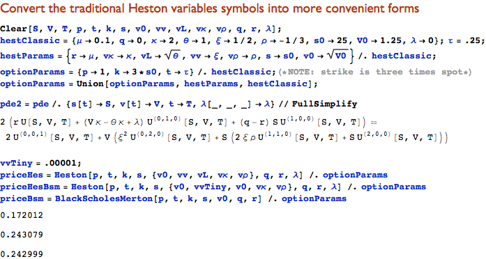
priceHes = Heston[p, t, k, s, {v0, vv, vL, vκ, vρ}, q, r,λ] /. optionParams

priceHesBsm = Heston[p, t, k, s, {v0, vvTiny, v0, vκ, vρ}, q, r,λ] /. optionParams

priceBsm = BlackScholesMerton[p, t, k, s, v0, q, r] /. optionParams

Print[TableForm[{{"BSM", "SemiAn Hest", "Sim Hest", "Sim Hest SE"},
  {priceBsm, priceHes, simHes, simHesSE}}]];


Out:=
0.172012

0.243079

0.242999

Derive the Heston PDE from the SDEs using BSM risk-neutral argument
(HELP!: I ran into trouble trying to render Mathematica's pd superscript format - can someone please provide a hint how to do it? I've left the mangled pd superscript code in this post just in case it's useful to someone...)
First, calculate the stochastic derivative of U(s,v,t) by taking the ItoProcess of the ItoProcess…
(Note: because ItoProcess reduces the processes to orthogonal rather then correlated wieners, we depart temporarily from the canonical derivations mentioned above)
Uproc = ItoProcess@ItoProcess[{
ds[t] == (μ - q) s[t]dt + Sqrt[v[t]] s[t]dws[t],

  dv[t] ==κ (θ - v[t])dt +ξ Sqrt[v[t]]dwν[t]},

  U[s[t], v[t], t], {{s, v}, {s0, v0}},
    t,
  {ws, wν}[Distributed] cW[ρ]];

dU = Last@ToSDEs[Uproc, {t, {ws, W}}];(*\W is a Wiener uncorrelated to ws*)

dU = Collect[dU,SuperscriptBox[U, TagBox[RowBox[{"(",
  RowBox[{"", ",", "", ",", "_"}], ")"}],Derivative],
  MultilineFunction->None][s[t], v[t], t]]
(The following is a GIF image of the above mangled expression)


Now, (unnecessarily) use the fact that dwν[t] =ρdws[t] + Sqrt[1 -ρ^2]dW[t] to reconstitute dwν[t] - this is just to show the SDE using the traditionally employed correlated "volatility" Wiener.
dU /.ξ ρ dws[t] Sqrt[v[t]] +ξ Sqrt[1 -ρ^2]dW[t] Sqrt[v[t]] ->ξ Sqrt[v[t]]dwν[t]

Now calculate dS and dU1...
Sproc = ItoProcess@ItoProcess[{
ds[t] == (μ - q) s[t]dt + Sqrt[v[t]] s[t]dws[t],

  dv[t] ==κ (θ - v[t])dt +ξ Sqrt[v[t]]dwν[t]},


  s[t], {{s, v}, {s0, v0}}, t,
  {ws, wν}[Distributed] cW[ρ]]


Out := ItoProcess[{{-q s[t] +μ s[t],θκ -κ v[t]},
  {{s[t] Sqrt[v[t]], 0}, {ξρ Sqrt[v[t]],ξ Sqrt[1 -ρ^2] Sqrt[v[t]]}},
  s[t]}, {{s, v}, {s0, v0}}, {t, 0}]
dS = First@ToSDEs[Sproc, {t, {ws, W}}](*\W is a Wiener uncorrelated to ws*)


Out:= dt (-q s[t] +μ s[t]) +dws[t] s[t] Sqrt[v[t]]
U1proc = ItoProcess@ItoProcess[{
ds[t] == (μ - q) s[t]dt + Sqrt[v[t]] s[t]dws[t],

  dv[t] ==κ (θ - v[t])dt +ξ Sqrt[v[t]]dwν[t]},

  U1[s[t], v[t], t], {{s, v}, {s0, v0}}, t,
  {ws, wν}[Distributed] cW[ρ]];

dU1 = Last@ToSDEs[U1proc, {t, {ws, W}}];(W is a Wiener uncorrelated to ws)

dU1 = Collect[dU1,SuperscriptBox[U1, TagBox[RowBox[{"(",

RowBox[{"", ",", "", ",", "_"}], ")"}],Derivative],
  MultilineFunction->None][s[t], v[t], t]]


Ito derivative, dΠ, of the derivative value, U[s[t],t], hedged with Δ of stock, s[t] and Δ1 of a 2nd instrument, U1[s[t],t]
, form a portfolio of one "short" derivative plus a "long" position of Δ units of stock, plus a "long" position of Δ2 units of another derivative with exposure to the stock and its volatility
Clear[Δ, V, s, v, r,σ,μ,κ,ξ, t, s0, w1, w2];

Π = U[s[t], v[t], t] -Δ s[t] -Δ1 U1[s[t], v[t], t];

dΠ = dU -Δ (dS + s[t] qdt) -Δ1 dU1 // FullSimplify
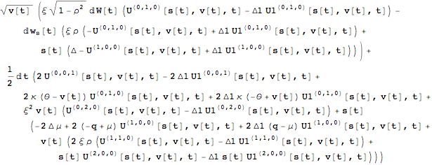
Extract the two risky components of dΠ, solve for Δ & Δ1, then substitute back into dΠ
eqnSrisk = dΠ /. {dt -> 0,dW[t] -> 0}

eqnWrisk = dΠ /. {dt -> 0,dws[t] -> 0}


find the values of Δ & Δ1 which completely hedges the stochasitic risk of the derivative
solnHedge = First@FullSimplify@Solve[eqnSrisk == 0 && eqnWrisk == 0, {Δ,Δ1}]

substitute Δ & Δ1 back into dΠ to make it "riskless" (by removing all the dw terms)
dΠ = FullSimplify[dΠ /. solnHedge]

Apply the risk-neutrality argument.
Now, because we've shown that the hedged portfolio is riskless, apply the Black-Scholes risk-neutrality argument and derive the Black-Scholes PDE by recognising that the return on the hedged portfolio must be the risk-free rate.
mma = r (Π /. solnHedge); (* risk-free money market account*)


lhs = FullSimplify[dΠ/dt - mma]; (*i.e. left hand side of dΠ-mma*)

pde = lhs == 0
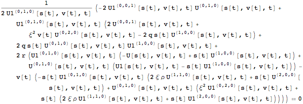
Collect the U and U1 terms to observe that each "side" is equivalent to some function of S, v & t
Clear[v];

pde = Collect[pde, {SuperscriptBox[U, TagBox[RowBox[{"(",
  RowBox[{"", ",", "", ",", ""}], ")"}],Derivative],
  MultilineFunction->None][s[t], v[t], t],
  SuperscriptBox[U1, TagBox[RowBox[{"(",
  RowBox[{"", ",", "", ",", ""}], ")"}],Derivative],
  MultilineFunction->None][s[t], v[t], t]}]

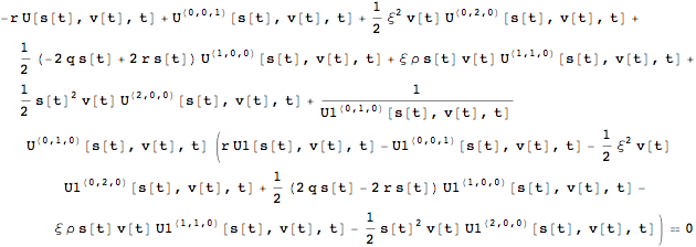
From the above, observe that collecting terms in U to one side of the equation, and U1 terms to the other, results in two equal expressions that have identical coefficients. Hence, we deduce that each expression is equal to the same equivalent function of S, v & t. So we arbitrarily define that equivalent function in terms of the expression containing only terms in the "extra" asset price, U1, and its greeks.
So, isolate the ∂U/∂v term from the above as the "equivalent function"...
Clear[equivFn];

equivFn = First[pde /.SuperscriptBox[U, TagBox[RowBox[{"(",
  RowBox[{"0", ",", "1", ",", "0"}], ")"}],Derivative],
  MultilineFunction->None][s[t], v[t], t] -> 1 /.SuperscriptBox[U,
  TagBox[RowBox[{"(",RowBox[{"", ",", "", ",", "_"}],
   ")"}],Derivative],MultilineFunction->None][s[t], v[t], t] -> 0
   /.SuperscriptBox[U, TagBox[RowBox[{"(", RowBox[{"0", ",", "0", ",", "0"}],
   ")"}],Derivative],MultilineFunction->None][s[t], v[t], t] -> 0]


Finally, replace the expression representing the "equivalent function" with an allowable functional form that includes what's called the "market price of volatility risk", λ ,to produce the final Heston PDE. λ is called the market price of volatility risk because it tells us how much of the expected return of U is explained by the risk (i.e. standard deviation) of v in the Capital Asset Pricing Model framework.
The "equivalent function" is chosen to also include the coefficient of the first derivative of v in the dΠ equation, before hedging. This completes the derivation of the Heston PDE.
Clear[α,β,λ];

pde = Collect[pde, {SuperscriptBox[U, TagBox[RowBox[{"(",
  RowBox[{"", ",", "", ",", ""}], ")"}],Derivative],
  MultilineFunction->None][s[t], v[t], t],
  SuperscriptBox[U1, TagBox[RowBox[{"(",RowBox[{"", ",", "", ",", ""}],
    ")"}],Derivative],
  MultilineFunction->None][s[t], v[t], t]}]
    /. {equivFn -> (κ (θ - v[t]) -λ[s[t], v[t], t])} // FullSimplify


Reformat the Heston PDE to more conventional form using a (slightly tweaked version of a) tool to be found on the web...
Clear[S];

FormatPDiff["Classic"];

pde /. {s[t] -> S, v[t] -> v}

FormatPDiff[];


Out := 2 (r U[S, v, t] + (v κ -θ κ +λ[S, v, t])∂U/∂v + (q - r) S ∂U/∂S)
  ==
 2 ∂U/∂t + v (ξ^2 ∂^2U/∂v^2 + S (2ξ ρ ∂^2U/∂S∂v + S ∂^2U/∂S^2))
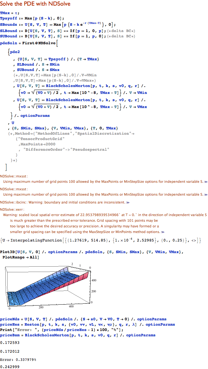
In a followup post I intend to explore a couple of things touched on above - maybe a comparison of the ItoProcess "Stochastic Runge-Kutta" vs. Andersen's "Quadratic-Exponential", and maybe using the derived PDE in NDSolve[ ]. Anyone else wants to jump in, too, please be my guest.


ItoProcess[], I'm setting this CW for the time being. $\endgroup$