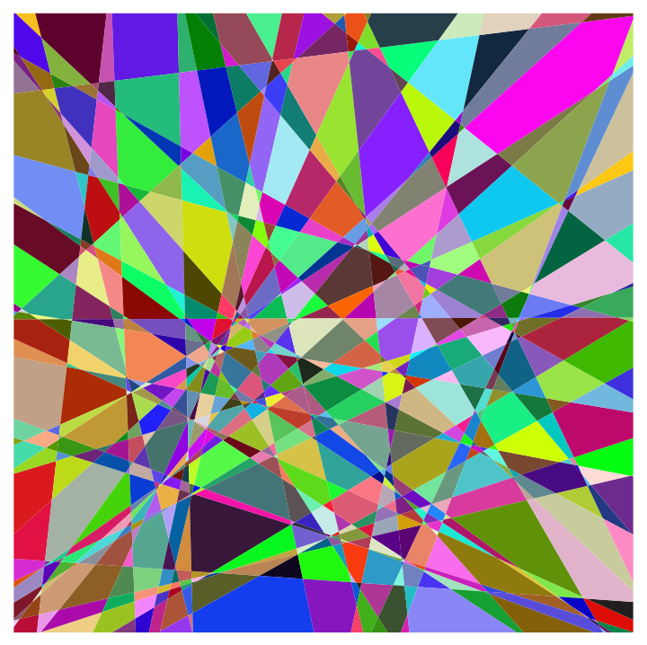
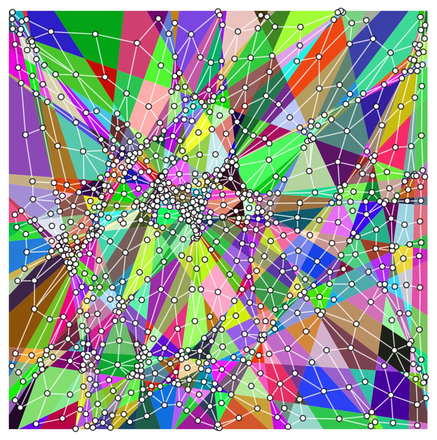
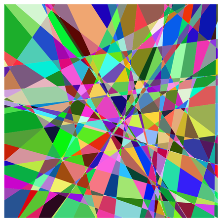
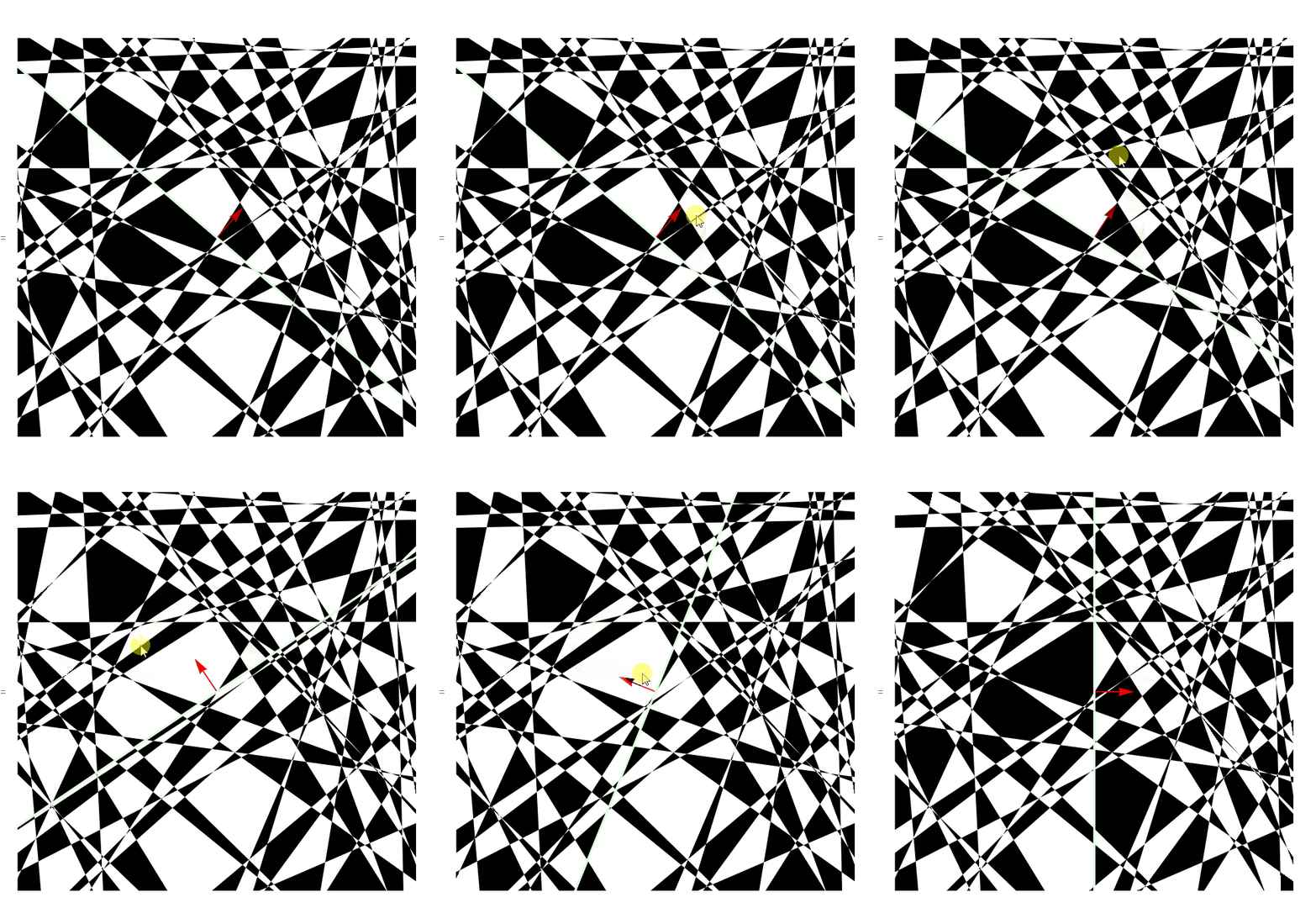
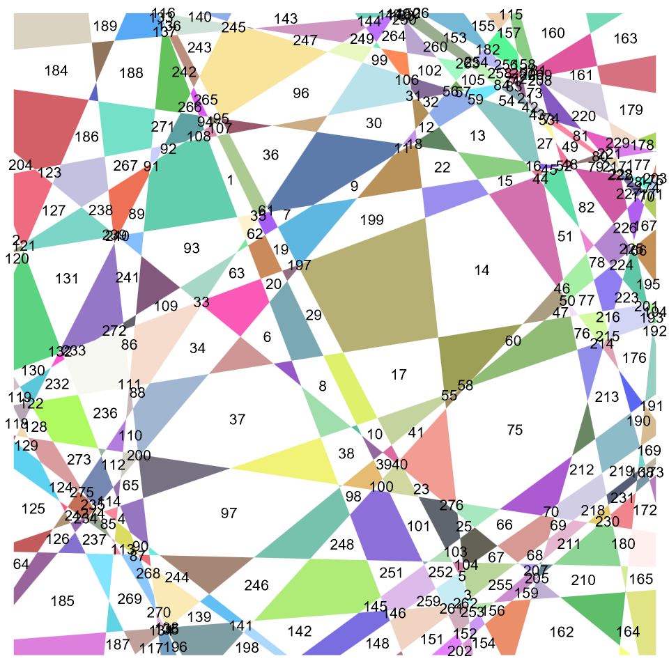
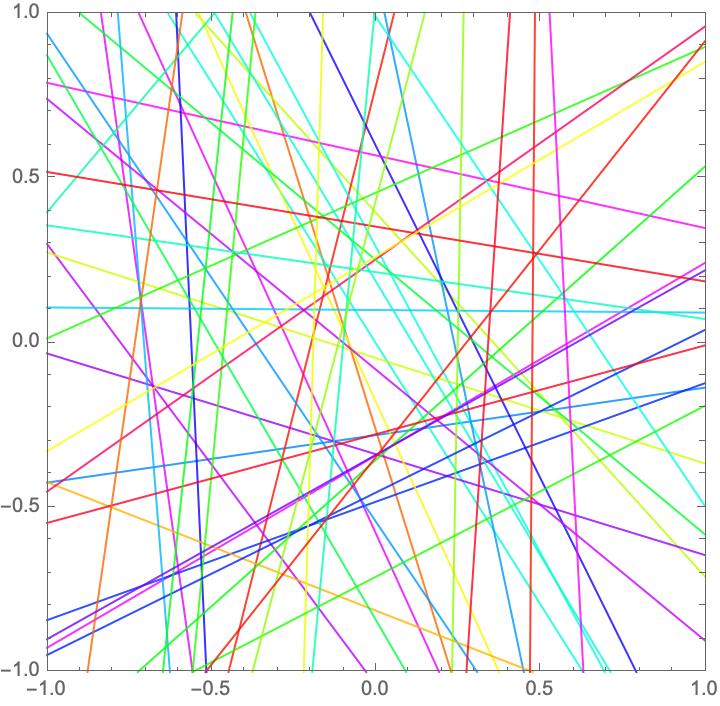
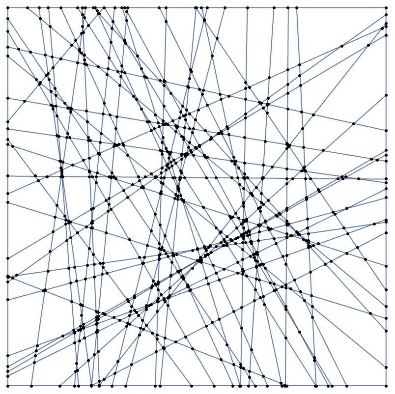
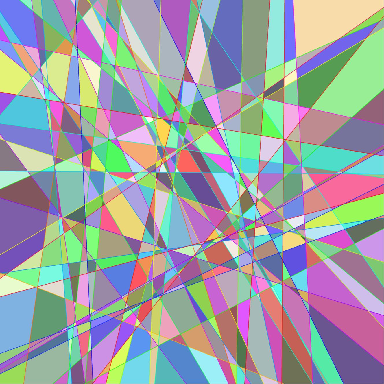
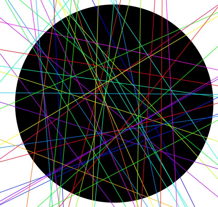
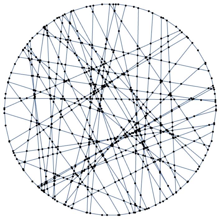
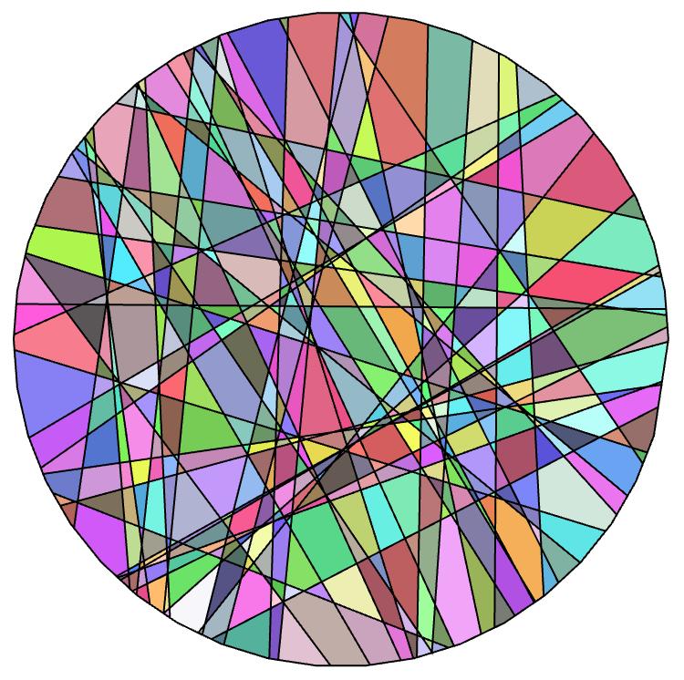
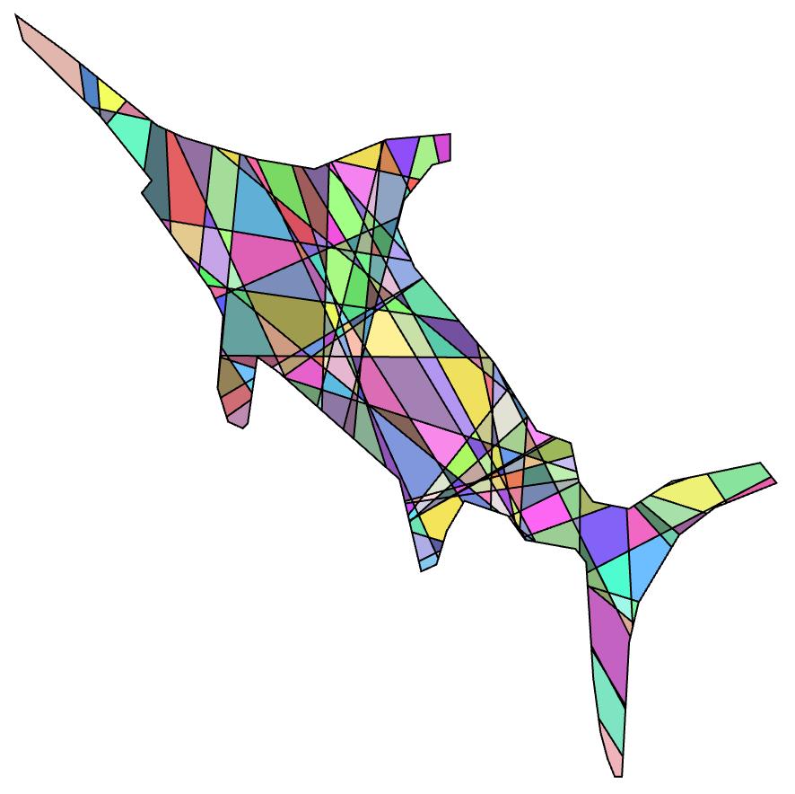
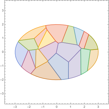
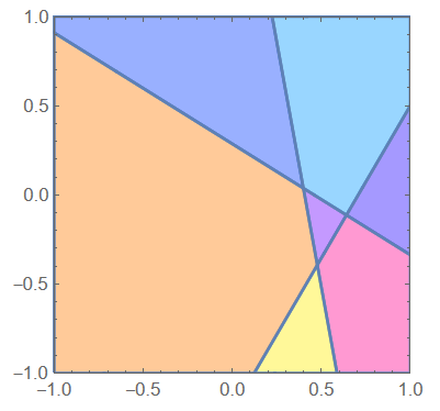
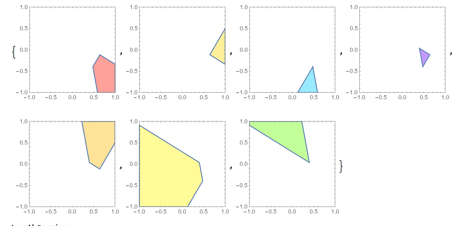
You can find symbolic connected components (which are those regions you are asking about) in this case using CylindricalDecomposition. This can be a bit of an overkill if your goal is only to visualize these regions between lines, but it is such a useful feature and extends to general semialgebraic sets, and thus I outline this solution and its extensions below.
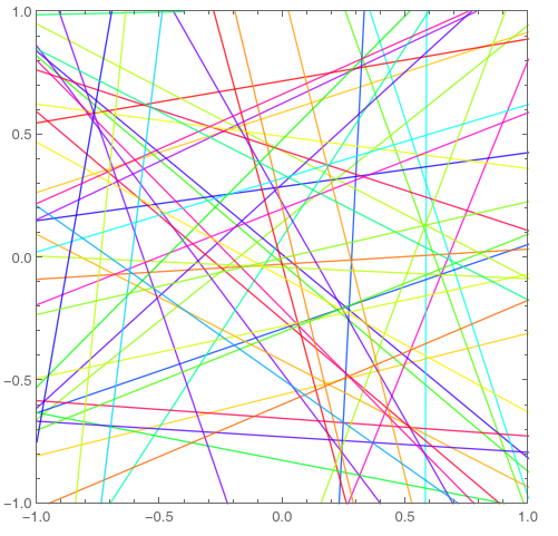
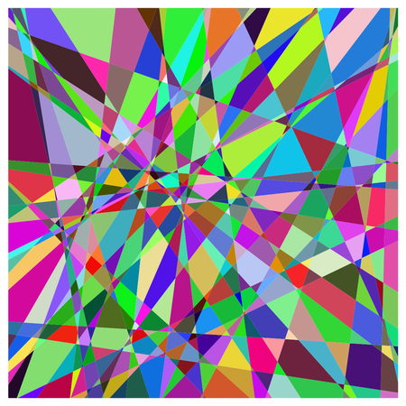
Below I first construct the rectangle and remove the lines (with rationalized random numbers) from it, splitting it to pieces. After this I compute equations representing these regions, and massage them a bit to make the input more palatable to CylindricalDecomposition which can extract the wanted regions using the "Components" topological operation. After this I reconstruct implicit regions from the resulting list of equations, discretize them, colour them randomly and show them.
RegionDifference[
     Rectangle[{-1, -1}, {1, 1}],
     RegionUnion@
      Table[InfiniteLine[Rationalize[RandomReal[{-1, 1}, {2, 2}], 0]], {49}]] //
    Refine[RegionMember[#, {x, y}], Element[x | y, Reals]] & //
   CylindricalDecomposition[#, {x, y}, "Components"] & //
  Map[Style[
     Quiet@BoundaryDiscretizeRegion@ImplicitRegion[#, {x, y}],
     RandomColor[]] &] // Graphics

This method is not fast for large numbers of lines, but CylindricalDecomposition can extract all components for these kind of problems, and the rest of the code visualises all of those which have nonzero area. One could improve this solution by two-colouring the result, but that's a different task.
EDIT:
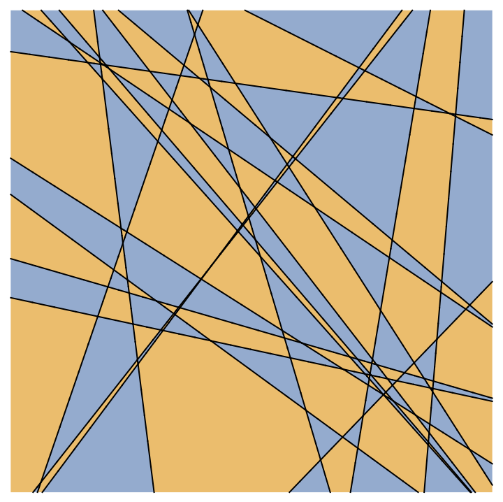
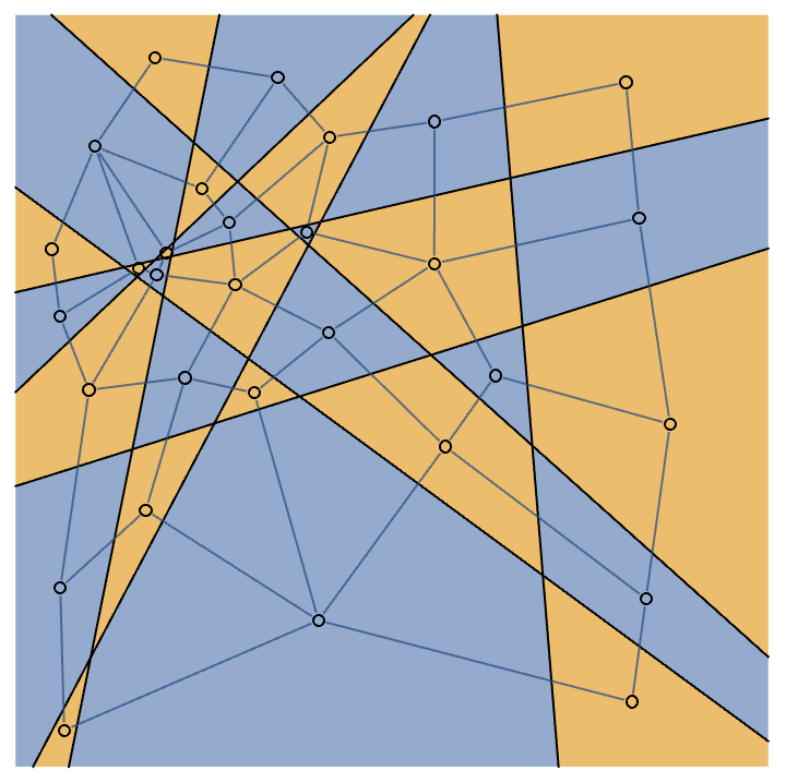
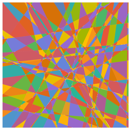
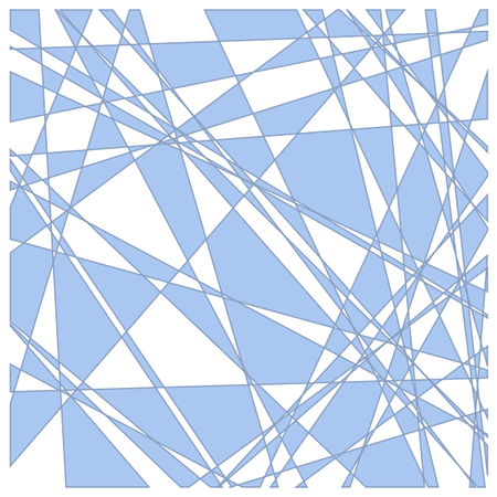
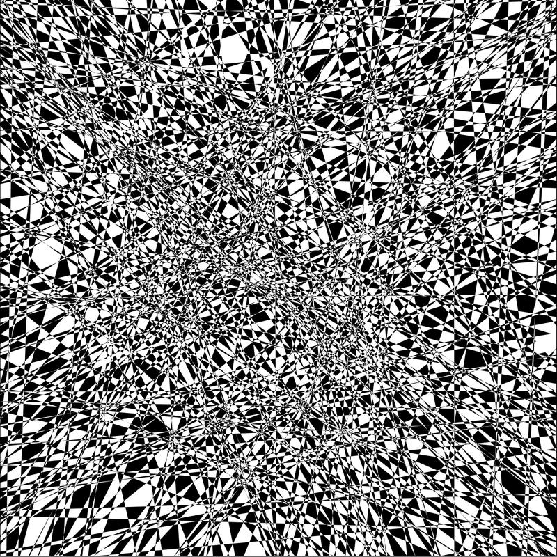
Although planar graphs are four-colourable, these graphs are two-colourable, meaning that only two colours are necessary to paint all regions with shared side with a differing colour. @cvgmt presents a fast method for two-colouring for this specific task using HalfSpaces and RegionSymmetricDifference, while the code below is more general purpose. (Unfortunately RegionSymmetricDifference can suffer from discretization issues, but that's another story - and I have a workaround for a similar problem below.)
Code below constructs symbolically the side-adjacency graph from a list of regions after splitting the region (as above) with a bit of trickery (the odd replacement rule could be replaced with CylindricalDecomposition[..., "Closure"], but that would result more complicated and thus more time-consuming operations down the line), and computes a colouring for it, visualising it in the end.
NOTE: Why did I comment out ParallelMap? Because apparently CylindricalDecomposition[..., "Components"] fails for many, if not all less trivial inputs on older Mathematica versions when parallel kernels are in use. This issue has been fixed in 13.1. You can effectively run this code with ParallelMap once on a fresh session, but not more than that.
With[{basereg = Rectangle[{-1, -1}, {1, 1}],
  lines =
   Table[InfiniteLine[Rationalize[RandomReal[{-1, 1}, {2, 2}], 0]], {20}]},
 RegionMember[RegionDifference[basereg, RegionUnion@lines], {x, y}] //
                          Refine[#, Element[x | y, Reals]] & //
            CylindricalDecomposition[#, {x, y}, "Components"] & //
           Map[ImplicitRegion[#, {x, y}] &] //
          (# /. {Greater ->
                GreaterEqual, GreaterEqual -> Greater,
              Less -> LessEqual, LessEqual -> Less}) & //
         Subsets[#, {2}] & //
        (*Parallel*)Map[
          Quiet@
            If[
             RegionDisjoint @@ # ||
              RegionDimension[RegionIntersection @@ #] == 0,
             Nothing, #] &, #] & //
       Map[Apply@UndirectedEdge] //
       SimpleGraph //
     {(*Parallel*)Map[Quiet@BoundaryDiscretizeRegion[#] &, VertexList[#](*,
        Method->"FinestGrained"*)],
       FindVertexColoring[#, Lighter@Take[ColorData[97, "ColorList"], 2]]} & //
    Transpose // Map[Apply@Style] //
  Graphics[{#,
     MeshPrimitives[
      DiscretizeRegion@RegionIntersection[basereg, RegionUnion@lines], 1]}] &]

It is also possible to visualise the graph which was used to generate the colouring:
With[{basereg = Rectangle[{-1, -1}, {1, 1}],
  lines =
   Table[InfiniteLine[Rationalize[RandomReal[{-1, 1}, {2, 2}], 0]], {8}]},
 With[{g =
    RegionMember[
             RegionDifference[basereg, RegionUnion@lines], {x, y}] //
                        Refine[#, Element[x | y, Reals]] & //
              CylindricalDecomposition[#, {x, y}, "Components"] & //
          Map[ImplicitRegion[#, {x, y}] &] //
         (# /. {Greater ->
             GreaterEqual, GreaterEqual -> Greater,
             Less -> LessEqual, LessEqual -> Less}) & //
        Subsets[#, {2}] & //
       (*Parallel*)Map[
         Quiet@
           If[
            RegionDisjoint @@ # ||
             RegionDimension[RegionIntersection @@ #] == 0,
            Nothing, #] &, #] & //
      Map[Apply@UndirectedEdge] //
     SimpleGraph[#, VertexShape -> Graphics@Circle[],
       VertexCoordinates -> (RegionCentroid /@ VertexList[#])] &},
  {(*Parallel*)Map[Quiet@BoundaryDiscretizeRegion[#] &, VertexList[g](*,Method->
       "FinestGrained"*)],
      FindVertexColoring[g, Lighter@Take[ColorData[97, "ColorList"], 2]]} //
     Transpose // Map[Apply@Style] //
   Show[Graphics[{#,
       MeshPrimitives[
        DiscretizeRegion@
         RegionIntersection[basereg, RegionUnion@lines], 1]}], g] &]]

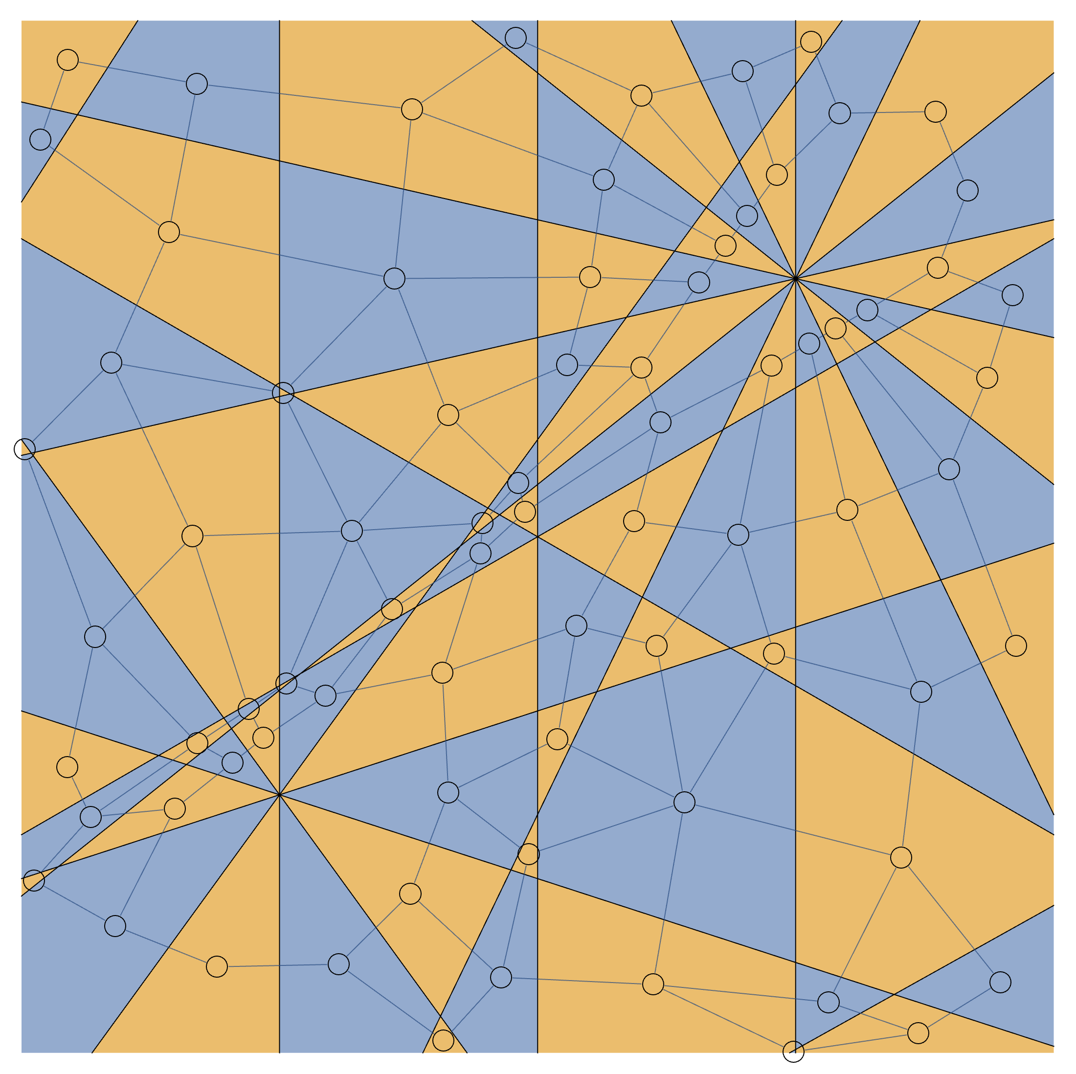
One more example with some less random lines:
lines = DeleteDuplicates@Join[
    Table[Rationalize[InfiniteLine[{0, 0}, N@{Sin[a], Cos[a]}], 0],
     {a, 0, 2 Pi, 2 Pi/3}],
    Table[
     Rationalize[InfiniteLine[-{1, 1}/2, N@{Sin[a], Cos[a]}], 0],
     {a, 0, 2 Pi, 2 Pi/5}],
    Table[Rationalize[InfiniteLine[{1, 1}/2, N@{Sin[a], Cos[a]}], 0],
     {a, 0, 2 Pi, 2 Pi/7}],
    Table[InfiniteLine[
      Rationalize[RandomPoint[Disk[{0, 0}, Sqrt[2]]], 0],
      Rationalize[RandomPoint[Circle[]], 0]], {2}]]}

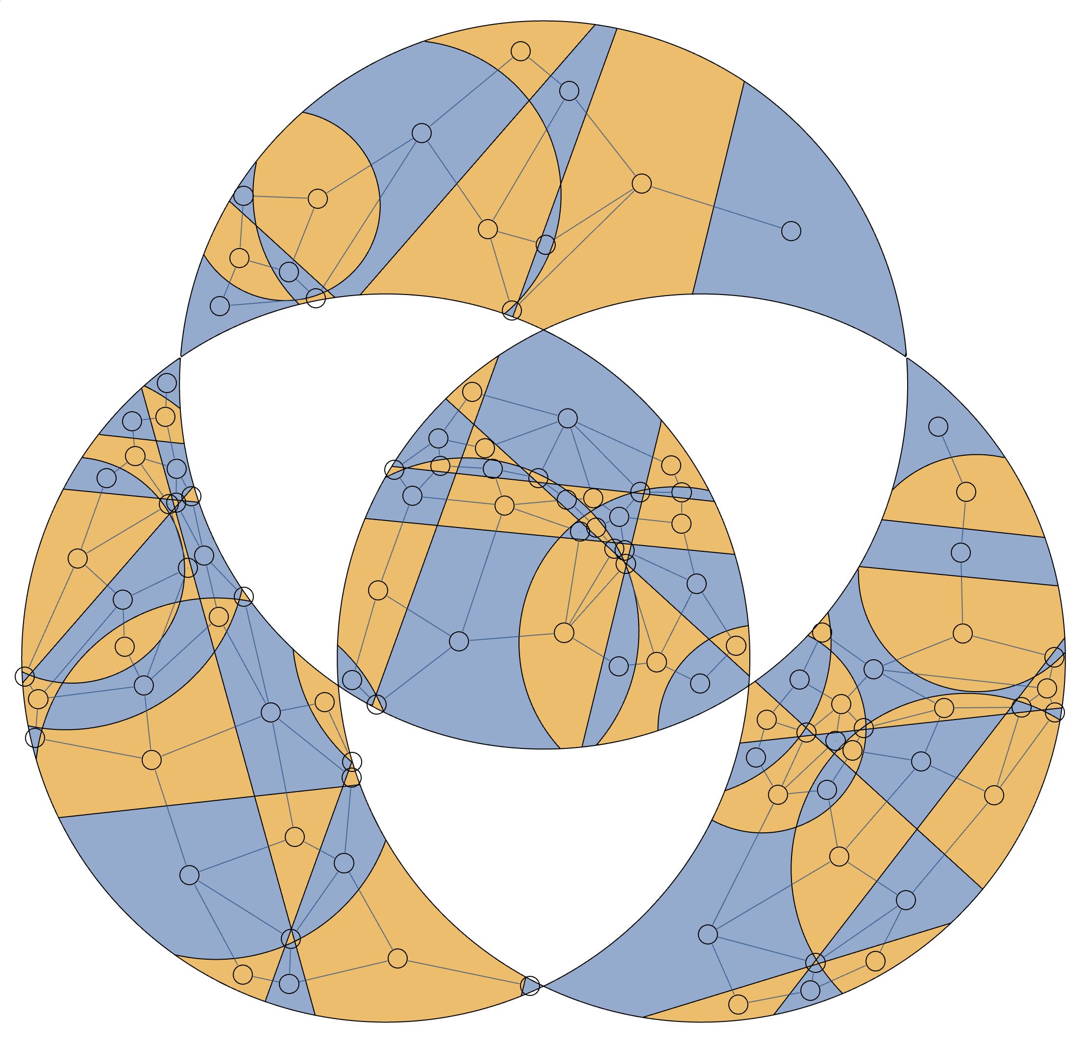
Technically speaking this approach is not limited to rectangles and lines, but can actually handle general semialgebraic sets. The process of getting good renderings and even getting the code to evaluate without running out of memory becomes more finicky in this case, though. For instance one should rationalize numbers at coarser accuracy and some hacks on discretizing implicit regions may be necessary.
Interestingly the hardest problem to work around seems to be discretizing cusps on implicit subregions completely. (This is done purely for visualization purposes.) My hack here is effectively rasterizing them.
Since intersections with Circles can produce non-convex regions (unlike plain InfiniteLines), RegionCentroid for VertexCoordinates may put the graph vertex outside its region. To hack around this, RegionCentroid and its closest corresponding point on the (discretized) region boundary are computed and the local minimum of SignedRegionDistance on the line defined by them is searched, starting between these points. This produces reasonably aesthetic results, usually keeping graph edges from intersecting, and generally better than just minimizing SignedRegionDistance which can put the point in quite an extreme spot on the region.
ClearAll[implicitRegionDiscretize];
implicitRegionDiscretize[reg_ImplicitRegion,
  bbox : {{x1_, x2_}, {y1_, y2_}}, step_] :=
 With[{f = Compile[{{x, _Real}, {y, _Real}},
     Evaluate[
      Boole@
       Refine[RegionMember[reg, {x, y}], Element[x | y, Reals]]],
     CompilationOptions -> {"ExpressionOptimization" -> True,
       "InlineCompiledFunctions" -> True},
     RuntimeAttributes -> {Listable}, RuntimeOptions -> "Speed",
     CompilationTarget -> "C"]},
  ImageMesh[Image@Table[f[x, y],
     {y, Reverse@Subdivide[N@y1, y2, Max[200, Round[(y2 - y1)/step]]]},
     {x, Subdivide[N@x1, x2, Max[200, Round[(x2 - x1)/step]]]}],
   Method -> "LinearSeparable", DataRange -> bbox]]

With[{basereg = RegionSymmetricDifference @@ Table[
     Disk[Rationalize[N[{Sin[a], Cos[a]}/2], 1/1000], 1],
     {a, 0, 5 Pi/3, 2 Pi/3}]},
 With[{lines = DeleteDuplicates@Join[Table[
       Circle[Rationalize[N[{Sin[a], Cos[a]}/2], 1/1000], 1],
       {a, 0, 5 Pi/3, 2 Pi/3}],
      Table[
       InfiniteLine[
        Rationalize[RandomPoint[basereg], 1/1000],
        Rationalize[RandomPoint[Circle[]], 1/1000]], {10}],
      Table[Circle[
        Rationalize[RandomPoint[basereg], 1/1000],
        Rationalize[RandomReal[{1/4, 1/2}], 1/1000]], {10}]],
   bbox = RegionBounds@basereg},
  With[{g =
     RegionMember[
                RegionDifference[basereg, RegionUnion@lines], {x, y}] //
               Refine[#, Element[x | y, Reals]] & //
              CylindricalDecomposition[#, {x, y}, "Components"] & //
             Map[ImplicitRegion[#, {x, y}] &] //
            (# /. {Greater -> GreaterEqual,
                 GreaterEqual -> Greater, Less -> LessEqual,
                LessEqual -> Less}) & //
           Subsets[#, {2}] & //
          ParallelMap[
            Quiet@
              If[
               RegionDisjoint @@ # ||
                RegionDimension[RegionIntersection @@ #] == 0,
               Sequence @@ #, #] &, #, Method -> "FinestGrained"] & //
         Replace[#, {l_List :> UndirectedEdge @@ l,
            r_ImplicitRegion :> UndirectedEdge[r, r]}, {1}] & //
           SimpleGraph //
       VertexReplace[#,
         Rule @@@
          Transpose@{VertexList[#],
            ParallelMap[
             implicitRegionDiscretize[#, RegionBounds@#, 1/1000] &,
             VertexList[#], Method -> "FinestGrained"]}] & //
      Graph[#, VertexShape -> Graphics@Circle[],
        VertexCoordinates ->(*Parallel*)Map[
          With[{a = RegionCentroid@#},
            With[{b = RegionNearest[RegionBoundary@#, a]},
             a + c (b - a) /.
              Last@
               Quiet@
                FindMinimum[
                 SignedRegionDistance[#, a + c (b - a)], {c, 1/2},
                 Method -> "PrincipalAxis"]]] &,
          VertexList[#]]] &},
   {VertexList[g],
       FindVertexColoring[g,
        Lighter@Take[ColorData[97, "ColorList"], 2]]} //
      Transpose // Map[Apply@Style] //
    Show[
      Graphics[{#,
        MeshPrimitives[
         DiscretizeRegion[
          RegionIntersection[basereg, RegionUnion@lines], bbox,
          MaxCellMeasure -> 1/10000, MeshQualityGoal -> "Maximal"],
         1]}], g] &]]]

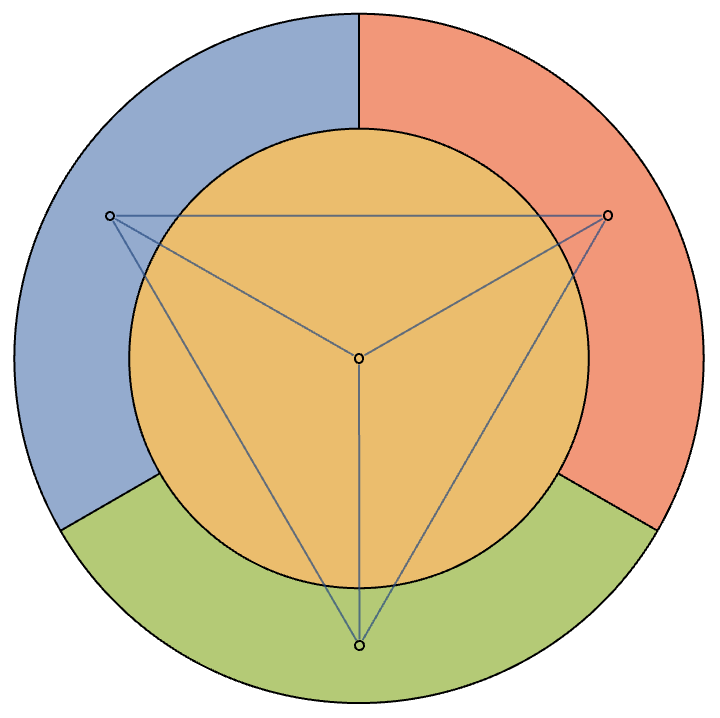
Just to prove that this also applies to a general-purpose colouring solution, use parameters below (produce a four-colouring):
$$\cdots$$
With[{basereg = Disk[]},
 With[{
   lines = {Circle[], Circle[{0, 0}, 2/3],
     Sequence @@ Table[
       Line[
        Rationalize[# {Sin@a, Cos@a} & /@ {1.9999/3, 1.0001},
         1/10000]],
       {a, 0, 5 Pi/3, 2 Pi/3}]},
   bbox = RegionBounds@basereg},
$$\cdots$$
{VertexList[g],
  FindVertexColoring[g, Lighter@Take[ColorData[97, "ColorList"], 4]]}  //
$$\cdots$$
