11
$\begingroup$

Say we have some functional like the following: $H = (\partial_yf(y))^2 -w(y) f(y)^2 +f(y)^4/2$. This is the functional for the Gross Pitaevskii equation. Lets say $w(y)$, the trapping potential in this case, is some simple inverted Gaussian just so we have an explicit equation to work with: $w(y) = e^{-y^2}$.

My question is, what efficient methods are available in Mathematica for finding the function $f(y)$ that minimizes this functional? I will outline two methods that I have found that are problematic, but I would love to know some alternatives!

Variational Methods

We can use the variational methods. So I define my function and use NDSolve to solve the Euler-Lagrange equation. One issue I have here is that I don't know apriori what constraints I should use: since this gives me a 2nd order differential equation, I need 2 constraints. I set the derivative at y=0 to be 0, as I expect f(y) to be symmetric about y=0. Since I want the functional to be minimized, I use the fact that $f'(0)=0$ to also come up with the constraint that $f(0) = 1$. (To get this, I simple plugged the first constraint into the functional and solved for $f(0)$ that minimized the functional).

Needs["VariationalMethods`"]
w[y_]:=E^(-(y)^2)
sol = NDSolve[{EulerEquations[f'[y]^2 - w[y]*f[y]^2 + f[y]^4/2, f[y], y] , f'[0] == 0,f[0]==1}, f, {y, -5, 5}]

However, the result I am getting is certainly not a minimum of the functional. If one plots the above solution, you see that $f(y)$ blows up as |y| increases, which clearly can not be minimizing the functional because the functional has a term that goes at $f(y)^4$ which should keep $f(y)$ from blowing up. Am I doing something incorrectly here? I believe the issue is that it's trying to find an extrema rather than a Minima, which is what I am specifically looking for. However I don't know how to force it to minimize. If there were some way to simple use NMinimize to get a function, that would be ideal.

Discretize and Minimize

The other method I came up with may be the worst(most inefficient) way one could do this. The idea is the discretize y into pieces of size $\epsilon$, and treat each f[y] as an independent variable. One must also discretize the derivative as $f'[y] = (f[y]+f[y+\epsilon])/\epsilon$. Then you can directly minimize the functional as a function of N variables. The issue is that, if I want to know $f(y)$ with any precision, I need to make $\epsilon$ small, which means I have a very large number of variables. Thus, the minimization takes a very long time. Here is example code applying this to the above functional:

numbSite = 100;
var = Table[Subscript[\[Psi], i], {i, 0, numbSite - 1}];
\[Epsilon] = .1;
sites = Table[-\[Epsilon]*numbSite/2 + \[Epsilon]*i, {i, 1,numbSite}];

Ham2[var_?(VectorQ[#, NumericQ] &)] :=
  Sum[((var[[i + 1]] - var[[i]])/\[Epsilon])^2, {i, 1, numbSite - 1}] - 
   Sum[(E^(-(-\[Epsilon]*numbSite/2 + \[Epsilon]*i)^2))*var[[i]]^2 , {i, 1, numbSite}] + 
(1/2)*Sum[var[[i]]^4, {i, 1, numbSite}];


min = FindMinimum[{Ham2[var]}, 
   Table[Subscript[\[Psi], i], {i, 0, numbSite - 1}], 
   MaxIterations -> 100];

p1 = ListPlot[
   Table[{sites[[i]], var[[i]]^2 /. min[[2]]}, {i, 1, numbSite}]];

This gives closer to the result I am expecting. It's still very slow when I make the number of sites large, but at least it is something.

I would love to hear any suggestions you have on solving this problem! Functionals of this form are very common in physics (due to the usefulness of the Landau-Ginzburg theory) and it would be great to have more efficient ways of minimizing them.

$\endgroup$

2 Answers 2

9
$\begingroup$

I'd typically go for "discretize and optimize".

Here is a quick and dirty implementation of this strategy that avoids all symbolic computation and that utilizes Sobolev gradient descent with respect to the $H^1$ inner product to speed up the computations. See also Can Mathematica solve Plateau's problem (...)? for a more sophisticated application of $H^1$ gradient descent.

(I have to sort of armwrestle FindMininum to convince it to use the correct gradient. But I cannot change FindMininum's stopping criterion, so I stop it manually.)

In this example, I impose Dirichet boundary conditions.

n = 2001;
a = -5.;
b = 5.;
h = (b - a)/(n - 1);
w[y_] := E^(-(y)^2)
y = Subdivide[a, b, n - 1];
\[Omega] = w /@ y;

stiffness = SparseArray[
   {Band[{1, 1}] -> 2./h, Band[{2, 1}] -> -1./h, 
    Band[{1, 2}] -> -1./h},
   {n, n}
   ];
stiffness[[1, 1]] = 1./h;
stiffness[[-1, -1]] = 1./h;

mass = SparseArray[
   {Band[{1, 1}] -> 2./3 h, Band[{2, 1}] -> 1./6 h, 
    Band[{1, 2}] -> 1./6 h},
   {n, n}
   ];
mass[[1, 1]] = 1./3 h;
mass[[-1, -1]] = 1./3 h;

ClearAll[F];
\[Omega] = Total[mass] w /@ y;


F[f_?VectorQ] := With[{f2 = f f},
   f . stiffness . f - \[Omega] . f2 + 0.5 f2 . mass . f2
   ];
F'[f_?VectorQ] := With[{f2 = f f},
   2. f . stiffness - 2. \[Omega] f + (2. f2 . mass) f
   ];

stiffnessWithDirichletBnd = stiffness;
stiffnessWithDirichletBnd[[1]] = SparseArray[{1} -> 1., {n}];
stiffnessWithDirichletBnd[[-1]] = SparseArray[{n} -> 1., {n}];
solver = LinearSolve[stiffnessWithDirichletBnd, Method -> "Banded"];

H1GradientWithDirichlet[f_?VectorQ] := Module[{b},
   b = F'[f];
   b[[{1, -1}]] = {0., 0.};
   solver[b]
   ];

f0 = ConstantArray[1., n];

f0[[1]] = 1.;
f0[[-1]] = 2.;

Block[{f},
  {min, fmin} = Quiet@FindMinimum[F[f], {f, f0},
     Gradient :> H1GradientWithDirichlet[f],
     Method -> "Gradient",
     MaxIterations -> 30
     ];
  fmin = f /. fmin
  ];

"H1 Residual" -> Sqrt[# . stiffness . # + # . mass . #] &[
 H1GradientWithDirichlet[fmin]]

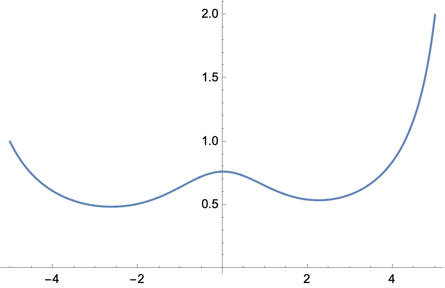
ListLinePlot[fmin, DataRange -> {a, b}, PlotRange -> All]

enter image description here

$\endgroup$
12
  • $\begingroup$ Thank you for the response, could you mention which functional you are minimizing here? From reading your code, I don't know what role stiffness and mass are meant to play, so it's not obvious to me how to edit the code to work with the functional I started with. $\endgroup$
    – Zonova
    Commented Apr 17, 2022 at 14:12
  • 1
    $\begingroup$ I tried to minimize the very functional that you posted. stiffness is the socalled stiffness matrix, Gram matrix of the $H^1$ scalar product with respect to the basis of piecewise-linear "hat functions". This way f.stiffness.f is a discretization of $\int_a^b (\partial_y f(y))^2 \, \mathrm{d} y$. mass is the so-called mass matrix, the Gram matrix of the $L^2$ scalar product so that f.mass.f discretizes $\int_a^b (f(y))^2 \, \mathrm{d} y$. $\endgroup$ Commented Apr 17, 2022 at 14:17
  • 1
    $\begingroup$ See also en.wikipedia.org/wiki/Stiffness_matrix. $\endgroup$ Commented Apr 17, 2022 at 14:22
  • 1
    $\begingroup$ Please try again; there were some definitions missing. \[Omega] . f2 or \[Omega] . (f f) computes the integral $\int_a^b w(y) \, (f(y))^2 \, \mathrm{d} y$. $\endgroup$ Commented Apr 17, 2022 at 17:35
  • 1
    $\begingroup$ I was wondering how one actually derives the stiffness and mass matrix. Here's how I would derive the functional to minimize. For the $\partial_y f^2$ term, I would use finite difference to get the derivative vector--let's call it $df$--where $df_i = (f_{i+1}-f_i)/h$. Then $\partial_y f^2 = df.df$. Then the other terms just come from something like f.f.f.f (this being taking the fourth power of y element wise). I am having a hard time understanding and finding a source on how to derive these stiffness and matrices. $\endgroup$
    – Tabin
    Commented May 5, 2022 at 17:03
3
$\begingroup$

The variational method produces a different solution, if the second boundary condition given in the question, f[0] ==1, is replaced by f[y] vanishing in the limit that y goes to infinity.

Needs["VariationalMethods`"]
w[y_] = E^(-(y)^2);
eq = MultiplySides[EulerEquations[f'[y]^2 - w[y]*f[y]^2 + f[y]^4/2,
    f[y], y], -1/2] // Expand
(* E^-y^2 f[y] - f[y]^3 + f''[y] == 0 *)

The desired solution is obtained by solving eq as a separatrix problem.

s = ParametricNDSolveValue[{eq, f'[0] == 0, f[0] == f0}, 
    f[y], {y, 0, 10000}, {f0}, WorkingPrecision -> 45];
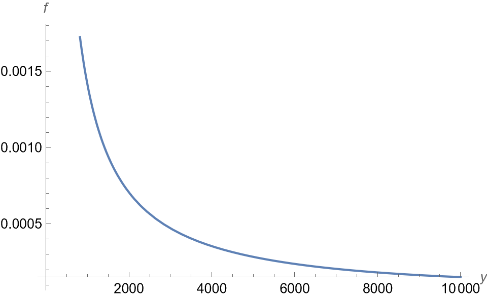
Plot[Evaluate[s[.731896481277023]], {y, 0, 10000}, AxesLabel -> {y, f}]

enter image description here

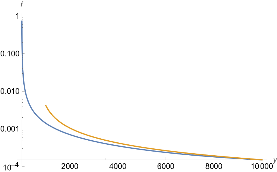
which I obtained by hand from successive guesses for the argument of s. This process can, of course, be automated, as in 147207. Comparing the result with the asymptotic solution show good agreement for large y,

sa = Simplify[DSolveValue[f'[y] == -f[y]^2/Sqrt[2], f[y], y] /. C[1] -> y0/Sqrt[2]]
(* Sqrt[2]/(y - y0) *)
sa /. Quiet@Solve[sa == s[.731896481277023] /. y -> 10000, y0] // First
(* Sqrt[2]/(-659.96456715484941226753617557390727253613055 + y) *)
LogPlot[{Evaluate[s[.731896481277023]], If[y > 1000, %]}, {y, 0, 10000}, 
    AxesLabel -> {y, f}, PlotRange -> All]

enter image description here

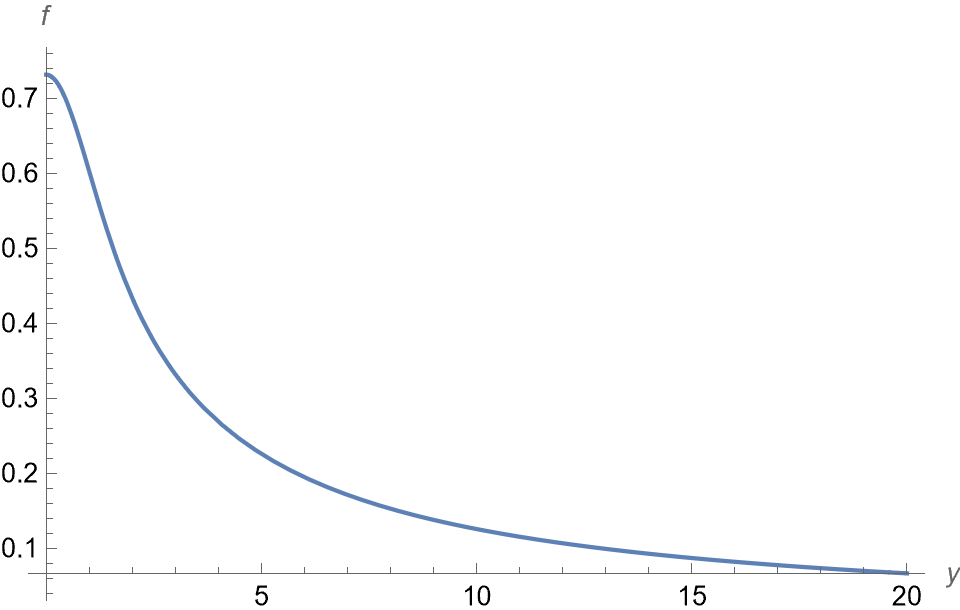
For completeness, here is a plot of the solution for small y.

Plot[Evaluate[s[.731896481277023]], {y, 0, 20}, PlotRange -> All, AxesLabel -> {y, f}]

enter image description here

Finally, the corresponding value of the integral of H is

sint = ParametricNDSolveValue[{eq, f'[0] == 0, f[0] == f0}, 
    f'[y]^2 - w[y]*f[y]^2 + f[y]^4/2, {y, 0, 10000}, {f0}, WorkingPrecision -> 45];
2 NIntegrate[Evaluate[sint[.731896481277023]], {y, 0, 10000}]
(* -0.334578 *)

This result is insensitive to the upper bound of the integral (e.g., 1000 instead of 10000. This integral clearly is smaller than that of the "Discretize and Minimize" result discussed in the question and in another answer. It also is smaller than the integral for the obvious analytical solution f[y] = 0.

$\endgroup$
3
  • $\begingroup$ Thank you for the answer! Apologies for the trivial question, but where/how are you imposing that f[y]->0 as y-> infinity? I can't seem to see that mentioned in the code $\endgroup$
    – Zonova
    Commented May 13, 2022 at 2:36
  • 1
    $\begingroup$ @Zonova The choice s[.731896481277023]] applies the boundary condition at large y. Varying the value from that just given produces solutions which diverge from zero at large y. $\endgroup$
    – bbgodfrey
    Commented May 13, 2022 at 13:05
  • $\begingroup$ @Zonova I thought that you had asked me another question, but I cannot find it. Is there another question that you had? $\endgroup$
    – bbgodfrey
    Commented May 15, 2022 at 2:05

Your Answer

By clicking “Post Your Answer”, you agree to our terms of service and acknowledge you have read our privacy policy.