2
$\begingroup$

I had a try at numerically solving the heat equation with a source term: $$ \frac{{\partial x}}{{\partial t}} = D\frac{{{\partial ^2}x}}{{\partial {z^2}}} + c $$

Manipulate[Module[{d, c, solN, pars, L0, pde, ic, bc, x, u, t}, L0 = 1;
  pde = D[u[x, t], t] == d D[u[x, t], {x, 2}] + c ;
  bc = {D[u[x, t], x] == 0 /. x -> 0, u[L0, t] == 0};
  ic = u[x, 0] == 1 - x;(*made up IC*)pars = {d -> d0, c -> c0};
  solN = Quiet@
    NDSolve[Evaluate[{pde, ic, bc} /. pars], 
     u, {x, 0, L0}, {t, 0, t0}];
  Quiet@Plot[Evaluate[u[x, t0] /. solN], {x, 0, L0}, 
    PlotRange -> {Automatic, {0, 1.5}}, GridLines -> Automatic, 
    GridLinesStyle -> LightGray, PlotStyle -> Red, 
    AxesLabel -> {"x", "u(x,t)"}, BaseStyle -> 12]], {{d0, 0.1, "D"}, 
  0.001, 1, 0.001, Appearance -> "Labeled"}, {{c0, 0, "c"}, 0, 10, 
  0.01, Appearance -> "Labeled"}, {{t0, 0, "time"}, 0, maxTime, 0.1, 
  Appearance -> "Labeled"}, {{maxTime, 200}, None}, 
 TrackedSymbols :> {d0, c0, t0}]

I messed up apparently because the bc2 is not doing what I want. Even if c=0 with time there is no diffusion.

Answer It requires a NeumannValue, to impose a basal flux=0:

Manipulate[
 Module[{d, c, solN, pars, L0, pde, ic, bc, x, u, t, \[CapitalGamma]},
   L0 = 1;
  pde = D[u[x, t], t] == 
    d D[u[x, t], {x, 2}] + c + NeumannValue[0, x == 0];
  bc = u[L0, t] == 0;
  ic = u[x, 0] == 1 - x;(*made up IC*)pars = {d -> d0, c -> c0};
  solN = Quiet@
    NDSolve[Evaluate[{pde, ic, bc} /. pars], 
     u, {x, 0, L0}, {t, 0, t0}];
  Quiet@Plot[Evaluate[u[x, t0] /. solN], {x, 0, L0}, 
    PlotRange -> {Automatic, {0, 1.5}}, GridLines -> Automatic, 
    GridLinesStyle -> LightGray, PlotStyle -> Red, 
    AxesLabel -> {"x", "u(x,t)"}, BaseStyle -> 12]], {{d0, 0.1, "D"}, 
  0.001, 1, 0.001, Appearance -> "Labeled"}, {{c0, 0, "c"}, 0, 10, 
  0.01, Appearance -> "Labeled"}, {{t0, 0, "time"}, 0, maxTime, 0.1, 
  Appearance -> "Labeled"}, {{maxTime, 200}, None}, 
 TrackedSymbols :> {d0, c0, t0}]

How to plot u[x,t] at x==0 as a function of t?

Tried:

Manipulate[
 Module[{d, c, solN, pars, L0, pde, ic, bc, x, u, t, \[CapitalGamma]},
   L0 = 5;
  pde = D[u[x, t], t] == 
    d D[u[x, t], {x, 2}] + c + NeumannValue[0, x == 0];
  bc = u[L0, t] == 0;
  ic = u[x, 0] == (L0 - x)/L0;(*made up IC*)pars = {d -> d0, c -> c0};
  solN = Quiet@
    NDSolve[Evaluate[{pde, ic, bc} /. pars], 
     u, {x, 0, L0}, {t, 0, t0}];
  Quiet@Plot[Evaluate[u[0, t0] /. solN], {t0, 0, 300}, 
    PlotRange -> {Automatic, {0, 1.5}}, GridLines -> Automatic, 
    GridLinesStyle -> LightGray, PlotStyle -> Red, 
    AxesLabel -> {"t", "u(0,t)"}, BaseStyle -> 12]], {{d0, 0.01, "D"},
   0.001, 1, 0.001, Appearance -> "Labeled"}, {{c0, 0, "c"}, 0, 10, 
  0.01, Appearance -> "Labeled"}, {{t0, 0, "time"}, 0, maxTime, 0.1, 
  Appearance -> "Labeled"}, {{maxTime, 300}, None}, 
 TrackedSymbols :> {d0, c0, t0}]

Write out the data for u[0,t]

Manipulate[
 Module[{d, c, solN, pars, L0, pde, ic, bc, x, u, t, \[CapitalGamma]},
   L0 = 5;
  pde = D[u[x, t], t] == 
    d D[u[x, t], {x, 2}] + c + NeumannValue[0, x == 0];
  bc = u[L0, t] == 0;
  ic = u[x, 0] == (L0 - x)/L0;(*made up IC*)pars = {d -> d0, c -> c0};
  solN = NDSolve[Evaluate[{pde, ic, bc} /. pars], 
    u, {x, 0, L0}, {t, 0, t0}];
(*data is GLOBAL so to access it from outside*)
data = Table[{t, Evaluate[u[0, t] /. solN]}, {t, 0, t0, 0.1}];
  Quiet@Plot[Evaluate[u[0, t] /. solN], {t, 0, t0}, 
    PlotRange -> {Automatic, {0, 1.5}}, GridLines -> Automatic, 
    GridLinesStyle -> LightGray, PlotStyle -> Red, 
    AxesLabel -> {"t", "u(0,t)"}, BaseStyle -> 12]], {{d0, 0.01, "D"},
   0.001, 1, 0.001, Appearance -> "Labeled"}, {{c0, 0, "c"}, 0, 10, 
  0.01, Appearance -> "Labeled"}, {{t0, 1, "time"}, 0.1, maxTime, 0.1,
   Appearance -> "Labeled"}, {{maxTime, 300}, None}, 
 TrackedSymbols :> {d0, c0, t0}]


Export[NotebookDirectory[] <> "data_table_test.csv", Flatten /@ data]
$\endgroup$
4
  • 2
    $\begingroup$ Hi @Dave, welcome to Mma.SE. To make the most of the site start by taking the tour now. It will help us to help you if you write an excellent question. Please edit your question if you can improve it, in this case to show due diligence, give brief context, include minimal working example of code you have tried. Have you read the documentation for NDSolve? what have you tried? $\endgroup$
    – rhermans
    Commented Nov 12, 2021 at 11:36
  • 1
    $\begingroup$ Well, as a beginner, the first thing you need to learn is, get used to reading the document of Mathematica, which is well-written and suitable for self-learning. As to your problem, NDSolve should be able to handle it without difficulty. $\endgroup$
    – xzczd
    Commented Nov 12, 2021 at 11:57
  • $\begingroup$ @rhermans I had a try at solving something simpler, and updated the question $\endgroup$
    – Dave
    Commented Nov 12, 2021 at 20:41
  • $\begingroup$ because the bc2 is not doing what I want. It not clear to me what you mean here. But Mathematica can solve this analytically and it has no problem. Below is an illustration. May be you could explain more that you think the problem is? btw, your Latex does not match the PDE. may be you can correct that. $\endgroup$
    – Nasser
    Commented Nov 12, 2021 at 22:42

2 Answers 2

4
$\begingroup$

I am not sure what the problem is, as it seems to be to be working ok.

But here is a version that uses DSolve (since it can solve this PDE analytically, then I see no reason to use NDSolve in this case, but this can be easily be changed)

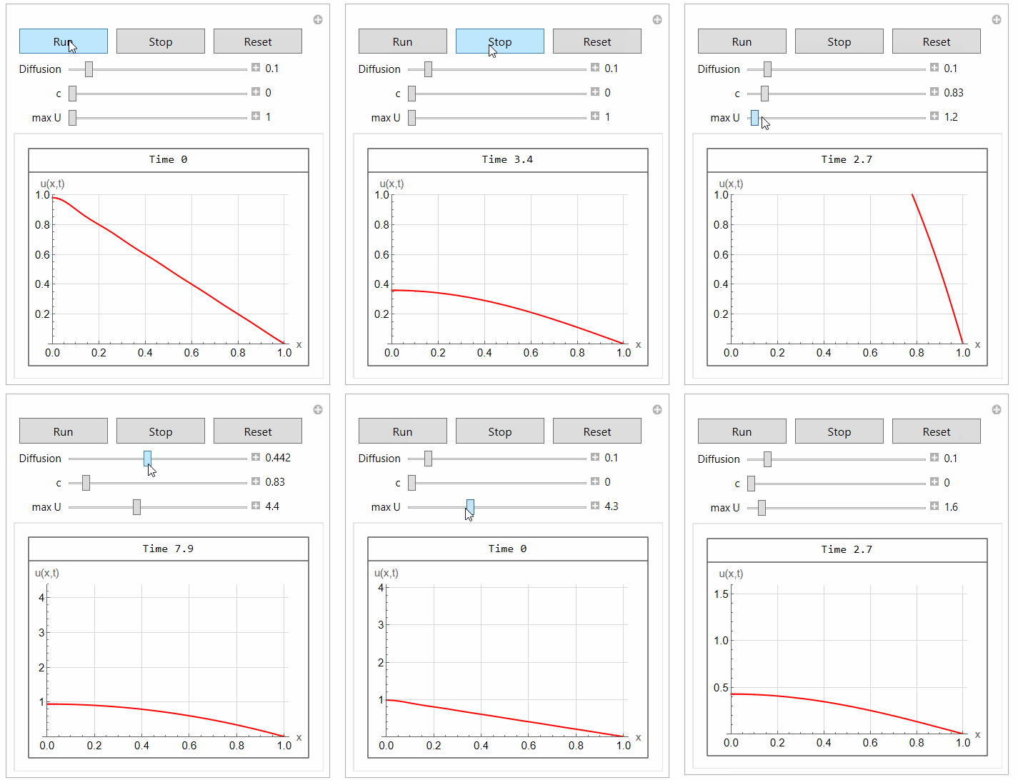
Added few buttons to make it easier to simulate. May be this will help you investigate the solution better.

enter image description here

First run this in separate cell to solve the PDE analytically.

Clear["Global`*"];
pde = D[u[x, t], t] == d*D[u[x, t], {x, 2}] + c;
bc = {D[u[x, t], x] == 0 /. x -> 0, u[L, t] == 0};
ic = u[x, 0] == 1 - x;(*made up IC*)
sol = DSolve[{pde, ic, bc}, u[x, t], {x, t}];
sol = u[x, t] /. First@Activate[sol /. {Infinity -> 10, K[1] -> n}];

enter image description here

etc.. The Analytical solution is a series. 10 terms are used. You can use more terms if you want. But I think this is enough for these kinds of problems.

And now in new cell, run Manipulate to use the above solution over and over. No need to solve the PDE each time. Solve it only once.

Manipulate[Module[{pars, L0},
  L0 = 1;
  pars = {d -> d0, L -> L0, t -> t0, c -> c0};
  If[state == "running",
   If [t0 < maxTime,
    t0 += 0.1; tick = Not[tick],
    t0 = 0
    ]
   ];
  Grid[{{Row[{"Time ", t0}]},
    {
     Quiet@Plot[sol /. pars, {x, 0, L0},
       PlotRange -> {Automatic, {0, maxU}},
       GridLines -> Automatic, GridLinesStyle -> LightGray,
       PlotStyle -> Red, AxesLabel -> {"x", "u(x,t)"},
       BaseStyle -> 12,
       ImageSize -> 300]
     }}, Frame -> All, Spacings -> {1, 1}]
  ],
 Grid[{
   {Button["Run", {state = "running"}, ImageSize -> 100],
    Button["Stop", {state = "stopped"}, ImageSize -> 100],
    Button[
     "Reset", {state = "stopped"; t0 = 0; c0 = 0; d0 = 0.1; 
      tick = Not[tick]}, ImageSize -> 100]
    }
   }
  ],
 {{d0, 0.1, "Diffusion"}, 0.001, 1, 0.001, Appearance -> "Labeled"},
 {{c0, 0, "c"}, 0, 10, 0.01, Appearance -> "Labeled"},
 {{maxU, 1, "max U"}, 1, 10, 0.1, Appearance -> "Labeled"},
 {{maxTime, 20}, None},
 {{tick, False}, None},
 {{t0, 0}, None},
 {{state, "stopped"}, None},
 TrackedSymbols :> {d0, c0, maxU, tick, state, t0}
 ]

How do I plot the u[x,0] = f(t) ? Which should look like an exponential decay for c=0, using NDsolve? I tried using the formulation I had initially but that plots u at x=0 as a straight line at all times

That is because your are plotting it at t=0 all the time! You are mixing symbols. You are doing Plot[Evaluate[u[0, t0] /. solN] but t0 is your control variable. Which is set to start at 0. That is why it does not change. Basically, you were doing this

Plot[1,{t0,0,300}]

Because Evaluate[u[0, t0] /. solN is 1

Try

Manipulate[
 Module[{d, c, solN, pars, L0, pde, ic, bc, x, u, t, \[CapitalGamma]},
  L0 = 5;
  pde = D[u[x, t], t] == 
    d D[u[x, t], {x, 2}] + c + NeumannValue[0, x == 0];
  bc = u[L0, t] == 0;
  ic = u[x, 0] == (L0 - x)/L0;(*made up IC*)
  pars = {d -> d0, c -> c0};
  solN = NDSolve[Evaluate[{pde, ic, bc} /. pars], 
    u, {x, 0, L0}, {t, 0, t0}];
  Quiet@Plot[Evaluate[u[0, t] /. solN], {t, 0, t0},
    PlotRange -> {Automatic, {0, 1.5}},
    GridLines -> Automatic, GridLinesStyle -> LightGray,
    PlotStyle -> Red,
    AxesLabel -> {"t", "u(0,t)"}, BaseStyle -> 12]
  ],
 {{d0, 0.01, "D"}, 0.001, 1, 0.001, Appearance -> "Labeled"},
 {{c0, 0, "c"}, 0, 10, 0.01, Appearance -> "Labeled"},
 {{t0, 1, "time"}, 0.1, maxTime, 0.1, Appearance -> "Labeled"},
 {{maxTime, 300}, None},
 TrackedSymbols :> {d0, c0, t0}
 ]

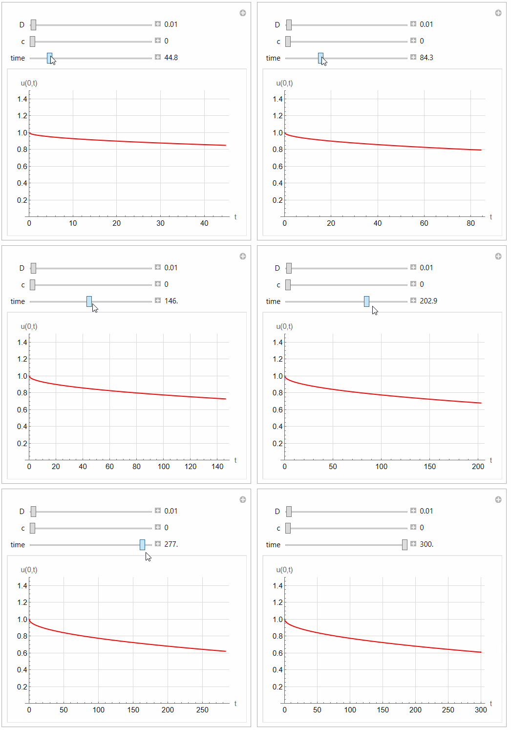
And you should not have t0 start at zero. Because Plot will complain if you have zero for length of plot. Try to make it little above zero.

enter image description here

Update to answer comment

How do I save the data in a csv? I tried this, but I cannot place them in the Manipulate data = Table[Evaluate[u[0, t] /. solN], {t, 0, 300, 0.1}]; Export["data_table_test.csv", data];

@Dave You are trying to use the solution and t0 from outside Manipulate. It does not "see" them, since solN is local to a module inside Manipulate. One way to work around this, is to save to the global data from inside Manipulate. Then in a new cell, you can now export it. But do not do Table[Evaluate[u[0, t] /. solN], {t, 0, 300,0.1}] from OUTSIDE, as it will not work and do not make data local variable to Manipulate.

Like this

Manipulate[
 Module[{d, c, solN, pars, L0, pde, ic, bc, x, u, t, \[CapitalGamma]},
   L0 = 5;
  pde = D[u[x, t], t] == 
    d * D[u[x, t], {x, 2}] + c + NeumannValue[0, x == 0];
  bc = u[L0, t] == 0;
  ic = u[x, 0] == (L0 - x)/L0;(*made up IC*)
  pars = {d -> d0, c -> c0};
  solN = NDSolve[Evaluate[{pde, ic, bc} /. pars], 
    u, {x, 0, L0}, {t, 0, t0}];
  (*data is GLOBAL so to access it from outside*)
  data = Table[Evaluate[u[0, t] /. solN], {t, 0, t0, 0.1}];
  Quiet@Plot[Evaluate[u[0, t] /. solN], {t, 0, t0}, 
    PlotRange -> {Automatic, {0, 1.5}}, GridLines -> Automatic, 
    GridLinesStyle -> LightGray, PlotStyle -> Red, 
    AxesLabel -> {"t", "u(0,t)"}, BaseStyle -> 12]], {{d0, 0.01, "D"},
   0.001, 1, 0.001, Appearance -> "Labeled"}, {{c0, 0, "c"}, 0, 10, 
  0.01, Appearance -> "Labeled"}, {{t0, 1, "time"}, 0.1, maxTime, 0.1,
   Appearance -> "Labeled"}, {{maxTime, 300}, None}, 
 TrackedSymbols :> {d0, c0, t0}]

And now in a new cell, you can use data

Mathematica graphics

And can now do anything you want with it. Notice each time you do something with Manipulate, the variable data will be updated automatically.

Update to answer comment

Can you show an example of this "button"?

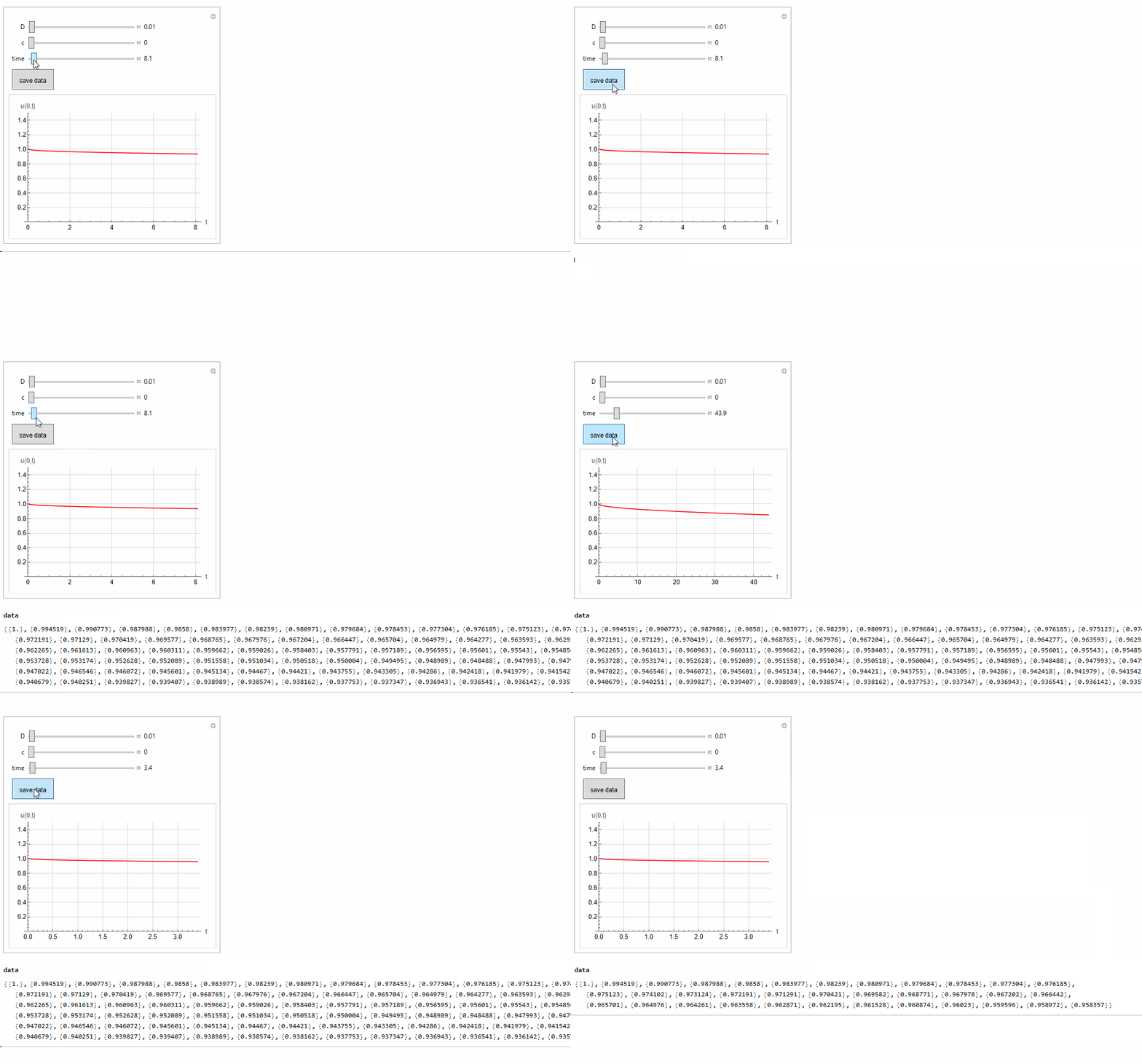
Here is a simple example. The data is saved only when you click on the button. This can be more efficient than saving it each time.

Manipulate[Module[{d, c, solN, pars, L0, pde, ic, bc, x, u, t}, 
  L0 = 5; 
  pde = D[u[x, t], t] == 
    d*D[u[x, t], {x, 2}] + c + NeumannValue[0, x == 0]; 
  bc = u[L0, t] == 0; 
  ic = u[x, 0] == (L0 - x)/L0; 
  pars = {d -> d0, c -> c0}; 
  solN = NDSolve[Evaluate[{pde, ic, bc} /. pars], 
    u, {x, 0, L0}, {t, 0, t0}]; 
  
  If[needToSaveData, 
   data = Table[Evaluate[u[0, t] /. solN], {t, 0, t0, 0.1}]; 
   needToSaveData = False]; 
  
  Quiet[Plot[Evaluate[u[0, t] /. solN], {t, 0, t0}, 
    PlotRange -> {Automatic, {0, 1.5}}, 
    GridLines -> Automatic, GridLinesStyle -> LightGray, 
    PlotStyle -> Red, AxesLabel -> {"t", "u(0,t)"}, 
    BaseStyle -> 12]]
  ], 
 
 {{d0, 0.01, "D"}, 0.001, 1, 0.001, Appearance -> "Labeled"}, 
 {{c0, 0, "c"}, 0, 10, 0.01, Appearance -> "Labeled"}, 
   {{t0, 1, "time"}, 0.1, maxTime, 0.1, Appearance -> "Labeled"}, 
 {{maxTime, 300}, None}, {{needToSaveData, True}, None}, 
   Grid[{{Button[
     Text[Style["save data", 12]], {needToSaveData = True}, 
     ImageSize -> {80, 40}]}}], 
 
 TrackedSymbols :> {d0, c0, t0, needToSaveData}
 
 ]

enter image description here

$\endgroup$
16
  • $\begingroup$ Thanks, it's awesome. Will this method also work if some terms are time-dependent? I would like D and c to be time-dependent in the next step $\endgroup$
    – Dave
    Commented Nov 13, 2021 at 0:01
  • $\begingroup$ @Dave probably not using DSolve if the coefficients are time dependent as then analytical solution might not be possible so have to go back to NDSolve $\endgroup$
    – Nasser
    Commented Nov 13, 2021 at 0:03
  • $\begingroup$ How do I plot the u[x,0] = f(t) ? Which should look like an exponential decay for c=0, using NDsolve? I tried using the formulation I had initially but that plots u at x=0 as a straight line at all times; @Nasser $\endgroup$
    – Dave
    Commented Nov 16, 2021 at 22:55
  • $\begingroup$ @Dave added note. $\endgroup$
    – Nasser
    Commented Nov 17, 2021 at 1:08
  • $\begingroup$ thanks a lot; learning so much thanks to those solutions you are sharing; @Nasser $\endgroup$
    – Dave
    Commented Nov 17, 2021 at 6:18
1
$\begingroup$

You should not ignore error messages like NDSolve::ibcinc: Warning: Boundary and initial conditions are inconsistent. >> with Quiet .

Change the derivative in bc to -E^(-t*10000), which is anytime very close to zero exept for t==0 and your first attempt works for me.

Manipulate[Module[{d, c, solN, pars, L0, pde, ic, bc, x, u, 
   t}, L0 = 1; pde = D[u[x, t], t] == 
      d*D[u[x, t], {x, 2}] + c; 
  bc = {Derivative[1, 0][u][0, t] == -E^((-t)*10000), 
      u[L0, t] == 0}; ic = u[x, 0] == 1 - x; 
  pars = {d -> d0, c -> c0}; 
  solN = NDSolve[Evaluate[{pde, ic, bc} /. pars], u, 
      {x, 0, L0}, {t, 0, t0}]; 
  Plot[Evaluate[u[x, t0] /. solN], {x, 0, L0}, 
    PlotRange -> All, GridLines -> Automatic, 
    GridLinesStyle -> LightGray, PlotStyle -> Red, 
    AxesLabel -> {"x", "u(x,t)"}, BaseStyle -> 12]], 
 {{d0, 0.1, "D"}, 0.001, 1, 0.001, 
 Appearance -> "Labeled"}, {{c0, 0, "c"}, 0, 10, 0.01, 
 Appearance -> "Labeled"}, {{t0, 0, "time"}, 0, maxTime, 
 0.1, Appearance -> "Labeled"}, {{maxTime, 200}, None}, 
 TrackedSymbols :> {d0, c0, t0}]
$\endgroup$
1
  • $\begingroup$ Thanks @Akku14 but your sol gives something a bit different. For instance at t=300 u[0,300] is 0.02 (t=5000, u[0,t] = 0.019; and with the NeumannValue bc u[0,300]=5E-4; $\endgroup$
    – Dave
    Commented Nov 19, 2021 at 1:12

Your Answer

By clicking “Post Your Answer”, you agree to our terms of service and acknowledge you have read our privacy policy.

Not the answer you're looking for? Browse other questions tagged or ask your own question.