1
$\begingroup$

This is not a completely Mathematica question, but I hope people who are familiar both with Mathematica and statistics could help me on this.

I have a set of data as

data = {{0, 0.046}, {40, 0.111}, {80, 0.291}, {120, 0.808}, {160, 1.742}, {200, 3.319}, {240, 5.017}, {280, 5.503}, {320, 5.897}}

The data seems to follow a logistic curve, thus for fitting, we can write:

F = NonlinearModelFit[data, A/(1 + E^(-(t - t0)/b)), {{A, 1}, {t0, 50}, {b, 10}}, t];
F["ParameterTable"]

Here is the result:

enter image description here

which is not bad, but I would like to improve it. Any suggestions here?

One thing the came to my head is to use inverse variances as weights. Standard deviations are given as

sd = {0.003, 0.012, 0.023, 0.056, 0.083, 0.216, 0.526, 0.366, 0.313}

thus, we have

F = NonlinearModelFit[data, A/(1 + E^(-(t - t0)/b)), {{A, 1}, {t0, 50}, {b, 10}}, t, Weights -> 1/sd^2];
F["ParameterTable"]

still, the results are not very satisfactory. Is there any other way to improve my fitting?

$\endgroup$
12
  • 1
    $\begingroup$ Looking at the plot, I think the curve fits pretty nicely to your datapoints. What exactly makes you think that the results are "not very satisfactory"? Which parameter are you considering? $\endgroup$
    – Domen
    Commented Aug 13, 2021 at 9:43
  • $\begingroup$ @Domen Thanks for your comment. The logistic rate of the plot, $1/b$, is $0.028$. I expected to be higher, for example, between $0.030$ and $0.035$, based on the expectations from the underlying mechanisms. I thought, perhaps, one could alter the logistic fitting to reproduce the mentioned values! $\endgroup$ Commented Aug 13, 2021 at 9:50
  • $\begingroup$ By using Manipulate[Show[ListPlot[Around[#[[1]], #[[2]]] & /@ Transpose[{data, sd}]], Plot[A/(1 + E^(-(t - t0)*b1)), {t, 0, 400}]], {{A, 6.26}, 4, 8}, {{t0, 197.7}, 160, 200}, {{b1, .025}, 0.02, 0.04}] and manually varying the parameters, you can see why $0.03$ gives a worse fit. This is even more pronounced if you use ListLogPlot and LogPlot, where the growth rate coincides with the slope of the line in the exponential phase of the growth (of course, using logarithmic plots can be a bit misleading, because the residuals are not equally scaled, but still). $\endgroup$
    – Domen
    Commented Aug 13, 2021 at 10:15
  • $\begingroup$ @Domen Many thanks for the above code, which is really helpful. Just a question: Could please elaborate how can I use ListLogPot and LogPlot for my data? $\endgroup$ Commented Aug 13, 2021 at 10:29
  • $\begingroup$ In the code I posted, replace ListPlot with ListLogPlot, and Plot with LogPlot. $\endgroup$
    – Domen
    Commented Aug 13, 2021 at 10:42

2 Answers 2

2
$\begingroup$

In your comments you mention that the responses are means of 3 values. If the response you're really interested in is the mean of 3 values, then we're ready to go. If the response should be the individual values and you really have a repeated measures design, then you should use something other than Mathematica. The functions LinearModelFit and NonlinearModelFit are just fine for simple models (with "simple" meaning just one error term).

To fit $k$ just replace $1/b$ with $k$. The underlying model that NonlinearModelFit thinks it's estimating is for the $i$-th observation

$$y_i=\frac{a}{e^{-k (t_i-t_0)}+1}+\epsilon_i$$

where $y_i$ is the response, $a$, $k$, and $t_0$ are parameters to be estimated, $t$ is the predictor variable and $\epsilon_i$ has a normal distribution with mean 0 and variance $\sigma^2$.

nlm1 = NonlinearModelFit[data, a/(1 + E^(-k (t - t0))), {{a, 1}, {t0, 50}, {k, 0.1}}, t];
nlm1["ParameterConfidenceIntervalTable"]

Parameter confidence interval table

We see that your desired 0.30 value for $k$ is included in the 95% confidence interval.

A plot of the predicted response vs the residuals suggests that the error term is incorrectly structured in that the variability seems to increase with an increase in predicted response.

ListPlot[Transpose[{nlm1["PredictedResponse"], nlm1["FitResiduals"]}]]
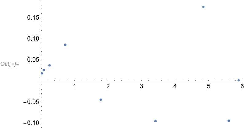
Predicted response vs residual

You also considered taking the logs of the responses.

data2 = data;
data2[[All, 2]] = Log[data2[[All, 2]]];
nlm2 = NonlinearModelFit[data2, Log[a/(1 + E^(-k (t - t0)))], {{a, 1}, {t0, 50}, {k, 0.1}}, t];
nlm2["ParameterConfidenceIntervalTable"]

Parameter confidence interval table for log transform

Note that your desired 0.30+ value for $k$ is not within a much tighter 95% confidence interval.

The residual plot doesn't display the increase in variability as before which suggests meeting the model assumptions better than the other model. In other words, this model provides a better fit to the data. It just doesn't provide a fit that coincides with your desires.

ListPlot[Transpose[{nlm2["PredictedResponse"], nlm2["FitResiduals"]}]]
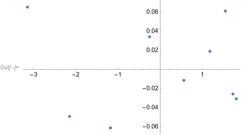
Residual plot from log transform

The data should really be analyzed according to how it was collected. And if the 3 values that constitute the means are available, that's what should be used in an analysis. But while one can use Mathematica to do so, that would entail a bit of programming as opposed to using NonlinearModelFit.

$\endgroup$
2
  • $\begingroup$ Many thanks! A question: you concluded that your second model is a better fit. Now, if we consider the inverse variances as weights, we can reproduce the values of $k$ and the confidence interval that you obtained in your second model. So, can one say in this way we can incorporate the errors? $\endgroup$ Commented Aug 13, 2021 at 23:14
  • $\begingroup$ If the weights are all the same value as you mentioned before ($1/\sqrt{3}$), then that won't change anything. $\endgroup$
    – JimB
    Commented Aug 13, 2021 at 23:19
1
$\begingroup$

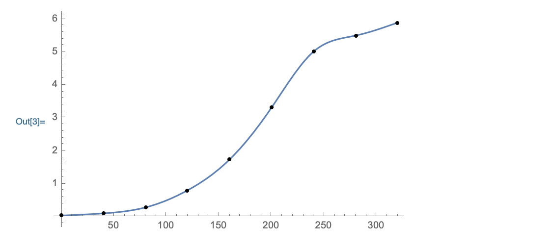
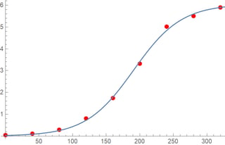
If you know the error in the data is essentially zero, you are better off with Monotonic-Interpolation in a case like this. The whole point of Interpolation is that the function you get goes exactly through each data point.

data=data={{0,0.046},{40,0.111},{80,0.291},{120,0.808},{160,1.742},
{200,3.319},{240,5.017},{280,5.503},{320,5.897}};
f=ResourceFunction["MonotonicInterpolation"][data];
Plot[f[t],{t,0,320},Epilog->{AbsolutePointSize@4,Point@data}]

plot If you want a closed form for the above function, use the next line.

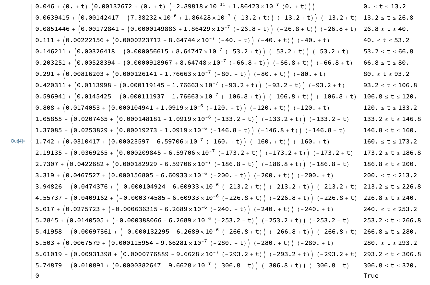
pw[t_] = ResourceFunction["InterpolatingFunctionToPiecewise"][f, t]

enter image description here

For more on the functions used above see documentation here and here.

Similar to MonotonicInterpolation there are ResourceFunctions here, here, and here that run faster on large datasets, but MonotonicInterpolation used above gives a smoother function.

***** UPDATE *****

Next I show how to find the maximum of the derivative of f[t] above.

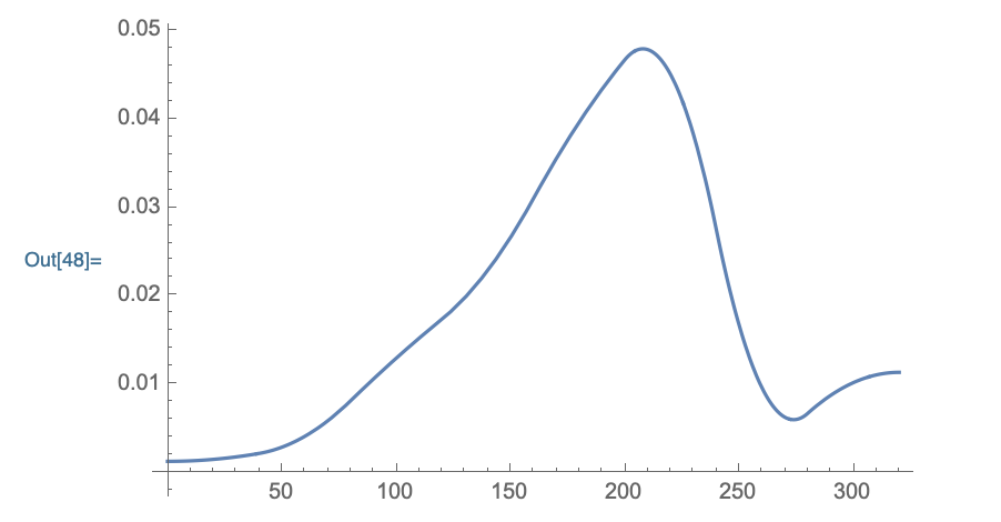
Plot[f'[t],{t,0,320}]

graphic Use a smaller PlotRange and it is clear the maximum of f'[t] is between 200 and 213. Look at the Piecewise function pw[t] defined above, and we see the interval from 200 to 213 is one piece of pw[t] and Simplify gives us that piece below.

poly=Simplify[pw[t],200<t<213]

cubic-polynomial Now we can find the maximum of the derivative of the above polynomial.

FindMaximum[D[poly,t],t]

maximum So in the plot of f'[t] above, the maximum derivative is at {t,f'[t]}={0.04799,207.91}

$\endgroup$
13
  • $\begingroup$ Wow, I never heard of this! Please let me time to understand your approach. Just two initial questions: I need to read off the "growth rate" from the curve. In your fitted curve, how can I do this? Another question is: So, in your approach you have not whatsoever taken into account the errors, correct? $\endgroup$ Commented Aug 13, 2021 at 20:43
  • $\begingroup$ @Aneternalstudent for the growth rate you'd just take the derivative of that giant polynomial. For the peak growth rate you'd want to maximize it. $\endgroup$
    – flinty
    Commented Aug 13, 2021 at 21:11
  • $\begingroup$ @flinty Thanks for your comment. You mean that, first I take derivative of say $f$ with respect to $t$ and then use FindRoot to obtain the solutions of $f' = 0$? $\endgroup$ Commented Aug 13, 2021 at 21:14
  • $\begingroup$ Any of the algorithms I mention as well as the Interpolation that Mathematica has built-in will return a function that perfectly passes through the data points. You could say I am assuming the errors are zero. However, if you want to nudge the curve in a certain direction, you can simply modify the data you pass to MonotonicInterpolation. That would give you a hand-wavy way of getting a smooth function that does whatever you want. As suggested by other comments, you can simply compute the derivative of the function that MonotonicInterpolation returns. $\endgroup$
    – Ted Ersek
    Commented Aug 13, 2021 at 21:36
  • 1
    $\begingroup$ Is this not likely a case of overfitting? Why would you not consider that there might be some measurement error? But wait...I see you start with an assumption that there is no error. Still...that seems extremely unlikely. $\endgroup$
    – JimB
    Commented Aug 13, 2021 at 21:50

Your Answer

By clicking “Post Your Answer”, you agree to our terms of service and acknowledge you have read our privacy policy.

Not the answer you're looking for? Browse other questions tagged or ask your own question.