1
$\begingroup$

I would like to create a 2D contour plot inside a closed region where the latter is produced by generating a parametric plot of a piecewise parametric function and then using BoundaryDiscretizeGraphics. If I plot each parametric component over its domain and then combine the plots with Show, the closed region is produced. However, if I use Piecewise to define the function and then produce the parametric plot, the closed region is not produced. I would much rather work with a single piecewise defined function, and thus would like to know what I am doing incorrectly. Any suggestion would be greatly appreciated. Below is a simple example of a triangular region that illustrates the problem.

With Piecewise

x[s_] = Piecewise[{{s, 0 <= s < 1}, {s, 1 <= s < 2}, {2 (3 - s), 
    2 <= s < 3}}]

y[s_] = Piecewise[{{s, 0 <= s < 1}, {2 - s, 1 <= s < 2}, {0, 
    2 <= s < 3}}]
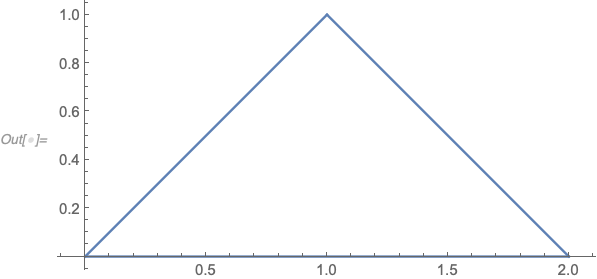
plot01 = ParametricPlot[{x[s], y[s]}, {s, 0, 3}]

enter image description here

BoundaryDiscretizeGraphics[plot01]

enter image description here

Without Piecewise

plot01 = ParametricPlot[{s, s}, {s, 0, 1}];
plot02 = ParametricPlot[{s, 2 - s}, {s, 1, 2}];
plot03 = ParametricPlot[{2 (3 - s), 0}, {s, 2, 3}];
plot04 = Show[{plot01, plot02, plot03}, PlotRange -> All]

enter image description here

BoundaryDiscretizeGraphics[plot04]
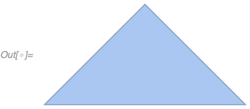
enter image description here

$\endgroup$

1 Answer 1

2
$\begingroup$

We need to use Exclusions -> None to contain the boundary point to make a cycle curve to construct a region.

x[s_] = Piecewise[{{s, 0 <= s < 1}, {s, 1 <= s < 2}, {2 (3 - s), 
     2 <= s < 3}}];
y[s_] = Piecewise[{{s, 0 <= s < 1}, {2 - s, 1 <= s < 2}, {0, 
     2 <= s < 3}}];
{plot01 = ParametricPlot[{x[s], y[s]}, {s, 0, 3}, Exclusions -> None],
  BoundaryDiscretizeGraphics[plot01]} // GraphicsRow

enter image description here

Edit

We can compare the two cases.

x[s_] = Piecewise[{{s, 0 <= s < 1}, {s, 1 <= s < 2}, {2 (3 - s), 
     2 <= s < 3}}];
y[s_] = Piecewise[{{s, 0 <= s < 1}, {2 - s, 1 <= s < 2}, {0, 
     2 <= s < 3}}];
plot01 = ParametricPlot[{x[s], y[s]}, {s, 0, 3}];
plot02 = ParametricPlot[{x[s], y[s]}, {s, 0, 3}, Exclusions -> None];
Cases[plot01, Line[a_] :> a, Infinity] 
Cases[plot, Line[a_] :> a, Infinity] 

( * plot01 *)
{{{0.0009566326530612245`, 
   0.0009566326530612245`}, ..., {0.9990433673469388`, 
   0.9990433673469388`}},
 {{1.0009566326530612`, 
   0.9990433673469388`}, ..., {1.9990433673469388`, 
   0.000956632653061229`}},
 {{1.998086734693878`, 0.`}, ..., {0.`, 0.`}}}
(* plot *)
{{{0., 0.},...,{0., 0.}}}
(* plot04 *)
{{{0.`, 0.`}, ..., {1.`, 1.`}},
 {{1.`, 1.`}, ..., {2.`, 0.`}},
 {{2.`, 0.`}, ..., {0.`, 0.`}}}

It means that plot is one cyclic curve and plot04 is end to end but plot01 just three independent curves and not end to end.

$\endgroup$

Your Answer

By clicking “Post Your Answer”, you agree to our terms of service and acknowledge you have read our privacy policy.

Not the answer you're looking for? Browse other questions tagged or ask your own question.