One needs to have a model (a predictive part and an error structure) to know what to do with the weights. If the weights are appropriate for the model, then one will tend to get better estimates of the parameters in the sense that the precision of the estimates will improve from not using weights. But one cannot judge the improvement just by looking at the overall change in fit from not using weights to using weights.
Consider the following model:
$$y_i={a \over{1+e^{-(t_i-t_0)/b}}}+w_i \epsilon_i$$
where $y_i$ is the $i$-th response, $t_i$ is the $i$-th predictor, $a$, $b$, and $t_0$ are constants to be estimated, the errors ($\epsilon_i$) are all independent, and $\epsilon_i \sim N(0,\sigma^2)$ for the $n$ observations with $i=1,2,\ldots,n$.
The Mathematica code for fitting such a model is as follows:
(* Data and weights *)
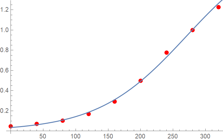
data = {{0, 0.047}, {40, 0.071}, {80, 0.103}, {120, 0.169}, {160, 0.292},
  {200, 0.498}, {240, 0.777}, {280, 1.000}, {320, 1.227}};
w = {0.003, 0.008, 0.010, 0.012, 0.023, 0.024, 0.061, 0.135, 0.221};

(* Fit *)
nlm = NonlinearModelFit[data, a/(1 + E^(-(t - t0)/b)), {{a, 1.2}, {t0, 200}, {b, 60}}, t,
  Weights -> 1/w^2]
mle = nlm["BestFitParameters"]
σ = nlm["EstimatedVariance"]^0.5
To check on whether using weights tends to result in better estimates for the parameters one can perform simulations. Suppose we use the estimated coefficients from your data as the "true" model. (But I'm reducing the size of the error variance to a tenth of the above estimate to avoid lack-of-convergence issues which can be especially problematic when the weights are ignored.)
(* Number of data points *)
n = Length[data];
(* Predictors *)
x = data[[All, 1]];
(* Scale down the variance to avoid lack-of-convergence issues *)
σ = 0.1 nlm["EstimatedVariance"]^0.5
(* Number of simulations *)
nsim = 200;

(* Generate mean prediction and errors *)
meanPrediction = a/(1 + Exp[-(x - t0)/b]);
errors = RandomVariate[NormalDistribution[0, σ], {nsim, n}];

(* Generate nsim datasets *)
datasim = meanPrediction + meanPrediction w # & /@ errors /. mle;
datasim = Transpose[{x, #}] & /@ datasim;

(* Now perform fits with and without weights *)
initialValues = {{a, (a /. mle)}, {b, (b /. mle)}, {t0, (t0 /. mle)}};
withWeights = {a, b, t0} /. NonlinearModelFit[#, a/(1 + Exp[-(t - t0)/b]),
  initialValues, t, Weights -> 1/w^2, MaxIterations -> 5000]["BestFitParameters"] & /@ datasim;
withoutWeights = {a, b, t0} /. NonlinearModelFit[#, a/(1 + Exp[-(t - t0)/b]),
  initialValues, t, MaxIterations -> 10000]["BestFitParameters"] & /@ datasim;
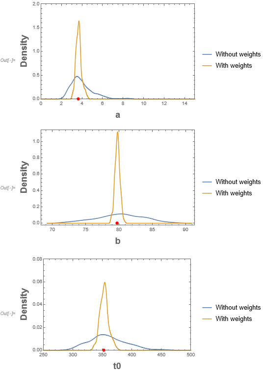
Now plot a smooth histogram of the estimates of each of the parameters with and without using weights:
Show[SmoothHistogram[{withoutWeights[[All, 1]], withWeights[[All, 1]]},
  Automatic, "PDF", PlotRange -> {{0, 15}, {0, 2}},
  Frame -> True, FrameLabel -> (Style[#, Bold, 18] &) /@ {"a", "Density"},
  PlotLegends -> {"Without weights", "With weights"}],
 ListPlot[{{a /. mle, 0}}, PlotStyle -> {{Red, PointSize[0.02]}}],
 PlotRangeClipping -> False]

Show[SmoothHistogram[{withoutWeights[[All, 2]], withWeights[[All, 2]]},
  Automatic, "PDF", Frame -> True, FrameLabel -> (Style[#, Bold, 18] &) /@ {"b", "Density"},
  PlotLegends -> {"Without weights", "With weights"}],
 ListPlot[{{b /. mle, 0}}, PlotStyle -> {{Red, PointSize[0.02]}}],
 PlotRangeClipping -> False]

Show[SmoothHistogram[{withoutWeights[[All, 3]], withWeights[[All, 3]]},
  Automatic, "PDF", PlotRange -> {{250, 500}, {0, .08}},
  Frame -> True, FrameLabel -> (Style[#, Bold, 18] &) /@ {"t0", "Density"},
  PlotLegends -> {"Without weights", "With weights"}],
 ListPlot[{{t0 /. mle, 0}}, PlotStyle -> {{Red, PointSize[0.02]}}],
 PlotRangeClipping -> False]

The red dots are the true values. One can see a great improvement by using weights (at least in this case where we know how the data was generated as used an estimation approach that matched the model). Much "tighter" estimates using weights.


