How to increase the speed of Collocation method to solve System of differential equations

Question

all. Kindly suggest me a ways to improve the speed of computations.
I recently came to know about collocation methods and their application to find solution for system of differential equations. Here I will describe the procedure in short. Bellow are the system of equations for 2D system.

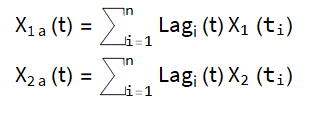
we will assume that we can represent the solution of above differential equations in terms of polynomials of some order n. We will divide the time(t) space into (n-1) so that we can have n point of discrete time, t(i) where i runs from 1 to n. Now we will assume some values of states X1 and X2 at these points. We can construct a polynomial using these data. In this problem I will be using Lagrange interpolation to approximate the states X1 and X2. These approximate states will be represented with X1a,X2a.

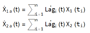
If we take first derivative for these approximate states (X1a,X2a) and equate it to original state derivatives at the discretized time points.

Since we initially assumed some values of X1,X2 at ti's . Now we will use NMinimize to find the values of X1,X2's at ti's. such that error is minimized. We can simplify this process and represent the final step as

Where D_lag is called as D matrix (Lagrange based D Matrix) and X1i is a column matrix of X1-initial guess values at discrete time ti's and X2i is a column matrix of X1-initial guess values at discrete time ti's. f1i and f2i are the value of actual functions evaluated at these discrete time points.

Here is my Mathematica work.

D matrix based on Lagrange can be calculate using this function

dMatrixLagrange[xpoints_] := Block[{ithDLagrangePCoeff, 
 dpLagrangList, x22, x, n}, n = Length[xpoints]; 
 ithDLagrangePCoeff[x_, j_] := 
  Sum[(1/(xpoints[[j]] - xpoints[[i]]))*
     Product[(x22 - xpoints[[m1]])/(xpoints[[j]] - 
        xpoints[[m1]]), {m1, Complement[Range[n], {i, j}]}], 
    {i, Complement[Range[n], {j}]}] /. x22 -> x; 
 dpLagrangList[x_] = (ithDLagrangePCoeff[x, #1] & ) /@ 
   Range[n]; (dpLagrangList[#1] & ) /@ xpoints];   

System of equations (We will compare Collocation method with NDSolve )

k = 5.;  
tf = 3.;
c[(θ1_)?NumericQ, (θ2_)?NumericQ] := NIntegrate[(Sin[θ1 + t]^2.*Cos[θ2 + t])/E^t, {t, 0., tf}];  

sol = NDSolve[{  
     Derivative[1][θ1][t] == θ2[t]/E^(Sin[t]/10.) + c[θ1[t], θ2[t]], 
     Derivative[1][θ2][t] == ((-k)*Sin[θ1[t]])/E^(Sin[t]/10.),  
     θ1[0.] == 1.,  
     θ2[0.] == 1.},  
    {θ1, θ2},  
    {t, 0., tf}]; 

Now discretizing the time points. Where npoints - number of time points needed. tpoints- list of time values, dotX- vector consists for first derivative functions

npoints = 11;
tpoints = Subdivide[0.0, tf, npoints - 1];
dotX[(arg_)?(VectorQ[#1, NumericQ] & )] :=Block[{t, θ1, θ2},  
  t = arg[[1]];  
 θ1 = arg[[2]];  
 θ2 = arg[[3]];  
 {  θ2/E^(Sin[t]/10.) + c[θ1,θ2], 
  ((-k)*Sin[θ1])/E^(Sin[t]/10.)  }  
];

Making discrete points symbolically

θ1aData = Table[ToExpression["θ1a" <> ToString[i]], {i, 1, 
Length[tpoints]}];  

 θ2aData = Table[ToExpression["θ2a" <> ToString[i]], {i, 1, 
Length[tpoints]}];  

θa1θ2aData = Transpose[{θ1aData, θ2aData}];  

tθa1θ2aData = Table[{tpoints[[i]], θ1aData[[i]], θ2aData[[i]]}, {i, 
1, Length[tpoints]}];

Making LHS side of equations

lhs1 = dMatrixLagrange[tpoints] . θa1θ2aData;

In order to use NMinimize we need objective function in a scalar form. So we take the Norm of LHS-RHS. Final form can be obtained using this function.

eqs[arg_?(VectorQ[#, NumericQ] &)] := Block[{s, sarg},
  s = Flatten[θa1θ2aData];  
  sarg = Partition[arg, 2];  
  Sqrt[Total[#^2 & /@ Flatten[(lhs1 /. Thread[s -> arg]) - Table[dotX[Flatten[{tpoints[[i]], 
  sarg[[i]]}]], {i, 1, Length[θa1θ2aData]}]]]]
  ];

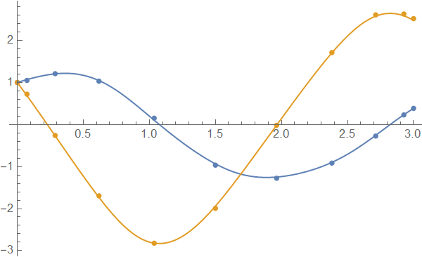
Using NMinimize and plotting the results and comparing with NDSolve result.

var = Flatten[θa1θ2aData];
rand = RandomReal[{-2, 2}, Length[var]]; 
initialG = MapThread[List, {var, rand}]; 
solnmin = NMinimize[{eqs[var], θ1a1 == 1., θ2a1 == 1.}, var];
tandθ1aData = Transpose[{tpoints, θ1aData}] /. solnmin[[2]]; 
θ1poly[x_] = InterpolatingPolynomial[tandθ1aData, x];
tandθ2aData = Transpose[{tpoints, θ2aData}] /. solnmin[[2]];
θ2poly[x_] = InterpolatingPolynomial[tandθ2aData, x];  

{  Plot[Evaluate[{θ1[t], θ1poly[t]} /. sol], {t, 0, tf}, PlotStyle -> Automatic, 
   PlotLegends -> {"θ1", "θ1a"}, AxesLabel -> {"t", "θ's"},  PlotLabel -> 
   StringJoin["Approximation m points ", ToString[Length[tpoints]], ", nth order ", 
   ToString[Length[tpoints] - 1]]],   
  Plot[Evaluate[{θ2[t], θ2poly[t]} /. sol], {t, 0, tf}, PlotStyle -> Automatic, 
  PlotLegends -> {"θ2", "θ2a"}, AxesLabel -> {"t", "θ's"}, 
   PlotLabel -> StringJoin["Approximation m points ", ToString[Length[tpoints]], ", nth order ", 
   ToString[Length[tpoints] - 1]]]
  }

results

This approach in Matlab and in Python took few minutes like about 3 minutes to get the result. The way I have written in Mathetmica code might be making the process very slow. to get this result it took me 30 minutes. Kindly suggest some way to speed up the process. Thanking you all.

Answer 1

First of all, the NDSolve solution can be further improved:

k = 5.;
tf = 3.; 
c[θ1_?NumericQ, θ2_?NumericQ] := 
  NIntegrate[(Sin[θ1 + t]^2. Cos[θ2 + t])/E^t, {t, 0., tf}, 
   Method -> {Automatic, SymbolicProcessing -> 0}];

sol = NDSolve[{θ1'[t] == θ2[t]/E^(Sin[t]/10.) + c[θ1[t], θ2[t]], 
               θ2'[t] == -k Sin[θ1[t]]/E^(Sin[t]/10.), 
     θ1[0.] == 1., θ2[0.] == 1.}, {θ1, θ2}, {t, 0., tf}]; // AbsoluteTiming
(* {0.0730725, Null} *)

ref = sol[[1, All, -1]] // ListLinePlot

Then, as to the implementation of collocation method, NMinimize is undoubtedly a bad choice. Just use FindRoot with the new-in-12.0 "AffineCovariantNewton" method. I've also turned to Chebyshev–Gauss–Lobatto grid to improve the accuracy of the solution:

CGLGrid[{xl_, xr_}, n_] := 1/2 (xl + xr + (xl - xr) Cos[(π Range[0, n - 1])/(n - 1)]);
  
npoints = 11;
tpoints = CGLGrid[{0., tf}, npoints];
myd = dMatrixLagrange[tpoints];

SetAttributes[c, Listable];
θ1init = {1.}; θ2init = {1.};
tst = FindRoot[{arg1, arg2} |-> 
                 With[{t = tpoints, θ1 = θ1init~Join~arg1, θ2 = θ2init~Join~arg2}, 
                      Rest /@ {myd . θ1 - (θ2/E^(Sin[t]/10.) + c[θ1, θ2]), 
                               myd . θ2 - (-k Sin[θ1])/E^(Sin[t]/10.)}], 
               {#, #} &@{ConstantArray[1., npoints - 1]}, 
               Method -> "AffineCovariantNewton"]; // AbsoluteTiming
(* {0.426819, Null} *)

ListPlot[{tpoints, #}\[Transpose] & /@ Join[{θ1init, θ2init}, tst, 2], 
  PlotRange -> All]~Show~ref

Remark

1. I've made use of the hidden syntax of FindRoot, a more basic approach is:

     help[arg1_List, arg2_] := 
      With[{θ1 = {1.}~Join~arg1, θ2 = {1.}~Join~arg2}, 
       Rest /@ With[{t = tpoints}, 
         {myd . θ1 - (θ2/E^(Sin[t]/10.) + c[θ1, θ2]), 
          myd . θ2 - (-k Sin[θ1])/E^(Sin[t]/10.)}]]
   
     tst = {arg1, arg2} /. 
      FindRoot[help[arg1, arg2], {#, ConstantArray[1., npoints - 1]} & /@ {arg1, arg2}]
   

2. NDSolve`FiniteDifferenceDerivative is a better choice to build myd e.g.:

   myd = NDSolve`FiniteDifferenceDerivative[1, tpoints, 
     DifferenceOrder -> 2]["DifferentiationMatrix"]
   
   NDSolve`FiniteDifferenceDerivative[1, tpoints, 
        DifferenceOrder -> "Pseudospectral"]["DifferentiationMatrix"] - 
      dMatrixLagrange[tpoints] // Abs // Max
   (* 2.66454*10^-14 *)
   

3. |-> is introduced in v12.2, if you're not yet in v12.2, use \[Function] instead.