8
$\begingroup$

I would like to plot the solution of the Fredholm Equation $$f\left(x\right)+\frac{1}{\pi} \int_{-1}^{1} \frac{1}{1+\left(x-t\right)^2}f\left(t\right) dt=1, \ \ (|x|\leq 1)$$ I tried to use Mathematica to find a numerical solution:

PHI = DSolveValue[\[Phi][x] == 1 - 1/Pi*Integrate[\[Phi][t]/(1 + (x - t)^2), 
      {t, -1, 1}], \[Phi], x]
Plot[PHI, {x, -1, 1}]

But I obtained some errors and I can't plot the numerical solution. How can I fix this problem?

$\endgroup$
6
  • $\begingroup$ In your Latex line there is one equation and in the Mathematica code there is second one. What actually do you try to solve? $\endgroup$ Commented Apr 4, 2021 at 23:03
  • $\begingroup$ Your code works for me for the DSolveValue part, but you won't get a plot without assigning a value for lambda. If you mean what you say in your code, you need to change your Latex to match. $\endgroup$
    – Bill Watts
    Commented Apr 5, 2021 at 0:40
  • $\begingroup$ Sorry everyone, I was wrong to copy the function in Mathematica. I corrected the post. $\endgroup$
    – Mark
    Commented Apr 5, 2021 at 6:34
  • $\begingroup$ Are you looking for analytical solution only? This equation can be solved by numerical method like colocation or iteration. $\endgroup$ Commented Apr 5, 2021 at 9:50
  • 1
    $\begingroup$ Just to compare. The command of Maple 2021 intsolve(f(x) + int(f(t)/(1 + (x - t)^2), t = -1 .. 1)/Pi = 1, f(x), method = collocation, order = 3) performs $$f \! \left(x \right) = 0.09775266381 x^{2}+ 0.6581514078 .$$ Analytical output is too long to be cited here. $\endgroup$
    – user64494
    Commented Apr 5, 2021 at 12:20

4 Answers 4

9
$\begingroup$

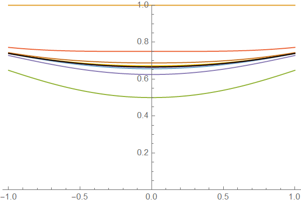
Perhaps NestList gives an iterated solution (Picard iteration)

sol = NestList[1 - 1/Pi*Integrate[#/(1 + (x - t)^2), {t, -1, 1},Assumptions -> -1 <= x <= 1] &, 0 , 10];    

Show[ Plot[sol  , {x, -1, 1}, PlotRange -> {0, 1}], 
Plot[sol[[-1]], {x, -1, 1}, PlotStyle -> {Thickness[.005], Black}]]

enter image description here

This gives the symbolic Neumann-Series .

$\endgroup$
5
  • $\begingroup$ As we know, for some Fredholm equations the iteration method is not converge at n->Infinity. It has minimal error at n about 6. What do you think about this equation? $\endgroup$ Commented Apr 5, 2021 at 12:48
  • $\begingroup$ @ AlexTrounev How did you check the error? If I compare the difference of two succesive iterations the numerical error seems to degree monoton. $\endgroup$ Commented Apr 5, 2021 at 12:58
  • 1
    $\begingroup$ The error is the difference between the true solution and an iterative one, not between two iterations. $\endgroup$ Commented Apr 5, 2021 at 14:17
  • $\begingroup$ @AlexTrounev But the true solution isn't known so far? $\endgroup$ Commented Apr 5, 2021 at 14:34
  • $\begingroup$ Yes it is. The true solution is known in theory only. $\endgroup$ Commented Apr 5, 2021 at 15:51
7
$\begingroup$

You have a wonderfully behaving smooth almost flat kernel. Since you want a numerical solution, then why not simply solve it with a quadrature?

To matrix equation with quadrature

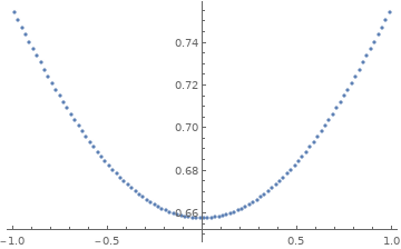
Here's a sample code in WolframAlpha notebook:

n=100;
K=Table[1/(1 + (2/n*(i - j))^2), {i,n}, {j, n}];
A=N[IdentityMatrix[n]+2/n*1/Pi*K];
f=LinearSolve[A,ConstantArray[1,n]];
ListPlot[N[Table[{2/n*(i -1/2)-1,f[[i]]}, {i,n}]]]
enter image description here

Here's how it works. Convert the integral equation into a matrix equation replacing the integral with the dumbest rectangle quadrature: $$\int K(x,t) f(t)dt=\sum_{i=1}^NK(x,t_i)f(t_i)\frac 2 N$$ where $t_i=2/N*(i-1/2)-1$.

Now, after plugging the same knots into $x$ variable you get a linear system: $$f_{t_i}+\frac 2 N \sum_jK_{t_it_j}f_{t_j}= \sum_j\left(\delta_{ij}+\frac 2 N K_{t_it_j}\right)f_{t_j}=1$$ $$\left(I+\frac 2 N K\right)f=\mathbf 1$$ which can be solved trivially with high precision as shown above.

Gauss-Legendre quadrature

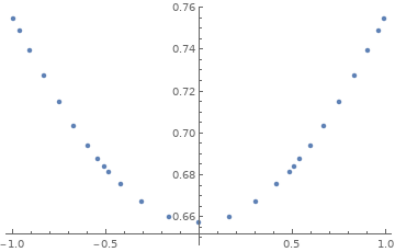
You can go fancy by employing Gaussian quadrature. Here's an example:

n = 27
<< NumericalDifferentialEquationAnalysis`;
knot = 0.5
gwL = GaussianQuadratureWeights[n/3, -1, -knot];
gwC = GaussianQuadratureWeights[n/3, -knot, knot];
gwR = GaussianQuadratureWeights[n/3, knot,1];
gw = Join[gwL,gwC,gwR];
n = Length[gw]

K=Table[1/(1 + ((gw[[i,1]] -gw[[j,1]]))^2)*gw[[j,2]], {i,n}, {j, n}];
A=N[IdentityMatrix[n]+1/Pi*K];
f=LinearSolve[A,ConstantArray[1,n]];
ListPlot[N[Table[{gw[[i,1]],f[[i]]}, {i,n}]]]

f[[Floor[n/2]+1]]

Out:     0.657412
enter image description here

Spectral decomposition

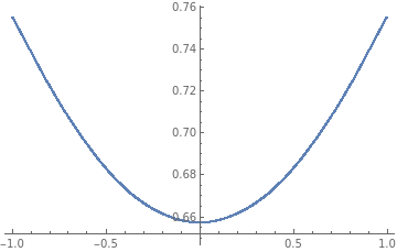
There is a different solution that gives an insight into the integral kernel. Apply the spectral decomposition to the kernel: $$-\frac 1 \pi \frac 1 {1+(x-t)^2}=\sum_{i=1}^\infty\lambda_i \psi_i(x)\psi_i(t)$$ Once you get the eigen values $\lambda_i$ and vectors $\psi_i(x)$, the solution to your problem is: $$f(x)\approx\sum_{i=1}^K \frac 1 {1-\lambda_i}\left(\int_{-1}^1\psi_i(t)dt\right)\psi(x)$$ , where $K$ is the number of eigenvectors used for approximation.
enter image description here

Usually, we order eigenvalues descending by absolute value. Because the kernel is smooth and almost flat only the first few eigenvalues are required because they decay so quickly: enter image description here
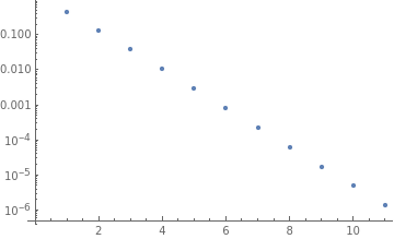
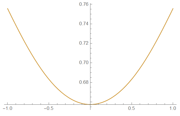
The first few eigen vectors are interesting to observe. The first one gets very close to the solution:
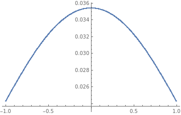
enter image description here

... and clearly only odd ones are symmetric and should have nonzero values of $\int_{-1}^1\psi_i(t)dt$ integral as shown next. Also, these integrals quickly decay too, helping to cut $K$, the number of required eigen vectors for high precision approximation:
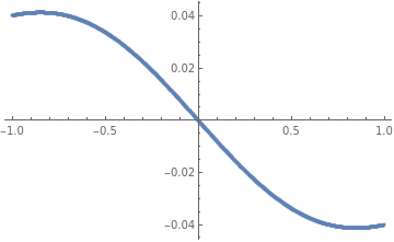
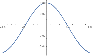
enter image description here enter image description here enter image description here

We can see now that if the right hand side wasn't simply a constant, 1 in your case, then a different - potentially larger - number $K$ of eigenvectors may have been required for a good approximation.

Here's the full code:

n=999;
x=N[Table[2*(i -1/2)/n-1, {i,n}]];
d=N[Table[1/(1 +(2/n* (i -j))^2)/Pi,{i,n},{j,n}]];
K = -d;
A=N[2/n*K];
{vals,v} = Eigensystem[A,11];

v1 = v[[1]]*Sum[v[[1,i]],{i,n}]/(1-vals[[1]]);
v3 = v[[3]]*Sum[v[[3,i]],{i,n}]/(1-vals[[3]]);
v5 = v[[5]]*Sum[v[[5,i]],{i,n}]/(1-vals[[5]]);
v7 = v[[7]]*Sum[v[[7,i]],{i,n}]/(1-vals[[7]]);
v9 = v[[9]]*Sum[v[[9,i]],{i,n}]/(1-vals[[9]]);
v11 = v[[11]]*Sum[v[[11,i]],{i,n}]/(1-vals[[11]]);
vapp = v1+v3+v5+v7+v9+v11;
ListPlot[Table[{x[[i]],vapp[[i]]},{i,n}]]

ListLogPlot[-vals]
ListPlot[Table[{x[[i]],v[[1,i]]}, {i,n}]]
ListPlot[Table[{x[[i]],v[[2,i]]}, {i,n}]]
ListPlot[Table[{x[[i]],v[[3,i]]}, {i,n}]]
ListPlot[Table[{x[[i]],v[[4,i]]}, {i,n}]]
$\endgroup$
6
$\begingroup$

One more colocation method based on Bernoulli (or Euler) polynomials with using NMinimize and FindRoot

 nN = 12; xcol = Table[-1 + 2 j/nN, {j, 0, nN}]; 
v[x_] := Table[BernoulliB[n, x], {n, 0, nN}]; A = Array[a, {nN + 1}]; 
u[x_] = A . v[x];
eqs = Table[
   u[xcol[[i]]] - 1 + 
    1/Pi A . 
      NIntegrate[v[t]/(1 + (xcol[[i]] - t)^2), {t, -1, 1}, 
       AccuracyGoal -> 8], {i, Length[xcol]}]; 

First method

sol = NMinimize[Norm[eqs], A]

Second method

sol1 = FindRoot[Table[eqs[[i]] == 0, {i, Length[eqs]}], 
  Table[{a[i], 1/10}, {i, Length[A]}]]

Visualization

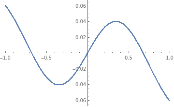
Plot[{u[x] /. sol1, u[x] /. sol[[2]]}, {x, -1, 1}]

Figure 1

$\endgroup$
6
  • $\begingroup$ For x=0 both methods yield 0.65741153600362792,but using method user @Ulrich Neumann give us 2/3.Which is correct one? $\endgroup$ Commented Apr 5, 2021 at 10:20
  • $\begingroup$ @MariuszIwaniuk Actually 2/3=0.66666..., and colocation method gives solution with some error of $h^2$. In my code h=1/12, so we have error of 1/144. $\endgroup$ Commented Apr 5, 2021 at 10:57
  • $\begingroup$ I tried with nN = 36 and give me: 0.6574115... ? $\endgroup$ Commented Apr 5, 2021 at 11:30
  • $\begingroup$ @MariuszIwaniuk Ah, I see, that your method also gives 0.657412 for n=10. May be true value is not 2/3? $\endgroup$ Commented Apr 5, 2021 at 12:07
  • 1
    $\begingroup$ Looks like at x=0 value is not 2/3.Try: N[Expand[DSolveValue[\[Phi][x] == 1 - 1/Pi* Integrate[\[Phi][ t]*(Series[1/(1 + (x - t)^2), {x, 0, 4}] // Normal) // Simplify // Expand, {t, -1, 1}], \[Phi][x], x]], 20] $\endgroup$ Commented Apr 5, 2021 at 15:50
6
$\begingroup$

Long ago I borrowed the code from site, but I don't know exactly where.

ClearAll["`*"]; Remove["`*"];

n = 5;
a1 = -1;
b1 = 1;
B[x_, i_] := Binomial[n, i]*((x - a1)^i*(b1 - x)^(n - i))/(b1 - a1)^n;
k[t_, x_] := -(1/(1 + (-t + x)^2));
a[x_] := 1;
f[x_] := 1;
\[Lambda] = 1/Pi;

nIntegrate[most__] := NIntegrate[most, Method -> {Automatic, SymbolicProcessing -> 0}];

K2[j_?NumericQ] := nIntegrate[B[x, j] f[x], {x, a1, b1}] // Quiet;
mid[x_?NumericQ, i_?NumericQ] := nIntegrate[\[Lambda] k[t, x] B[t, i], {t, a1, b1}] // Quiet;

K3[j_?NumericQ, i_?NumericQ] := 
nIntegrate[(a[x] B[x, i] - mid[x, i]) B[x, j], {x, a1, b1}] // Quiet;

sol = Table[Total@Table[M[i] K3[j, i], {i, 0, n}] == K2[j], {j, 0, n}];

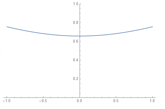
func = Total@Table[M[i] B[x, i], {i, 0, n}] /. NSolve[sol, Table[M[i], {i, 0, n}]][[1]]

Plot[func, {x, -1, 1}, PlotRange -> {Automatic, {0, 1}}]

enter image description here

$\endgroup$
3
  • $\begingroup$ Some hours ago there was a tricky numerical solution at the end of your answer , why did you delete it? $\endgroup$ Commented Apr 5, 2021 at 13:05
  • $\begingroup$ @Ulrich Neumann I'm not sure it was correct. $\endgroup$ Commented Apr 5, 2021 at 13:59
  • $\begingroup$ What a pity I was hoping it would be something like the "Method of lines for DAE systems"! What was wrong? $\endgroup$ Commented Apr 5, 2021 at 14:03

Your Answer

By clicking “Post Your Answer”, you agree to our terms of service and acknowledge you have read our privacy policy.

Not the answer you're looking for? Browse other questions tagged or ask your own question.