2
$\begingroup$

Is there a way to create an x coordinate and corresponding time table instead of having them automatically plotted for this wolfram demonstration https://demonstrations.wolfram.com/MassBetweenTwoDampedSprings/

I tried this answer: Plot, extract data to a file and added

data = Cases[Plot[d@t, {t, 0, 2 Pi}], Line[data_] :> data, -3, 3][[1]];

at the very bottom of the source code. But, when I opened the file it was rather empty.

How can I fix this?

EDIT (after following the first answer solution)**

I would want my resulting text file to look like:

1.2822827157509358e-7   1.2822827157509324e-7
0.0019271655319089223   0.001927164339004283
0.0038542028355462695   0.00385419329326691
0.007708277442820964    0.007708201108565738

But, what I have now is

IconizedObject[{{-0.1, -1.9539279806250676}, {-0.099, -1.9548413477229447}, {-0.098, -1.9557456736830732}, {-0.097, -1.9566409543229473}, {-0.096, -1.9575271855018952}, {-0.095, -1.9584043631210997}, {-0.094, -1.9592724831236157}, {-0.093, -1.9601315414943898}, {-0.092, -1.9609815342602783}, {-0.091, -1.9618224574900667}, {-0.09000000000000001, -1.9626543072944862}, {-0.08900000000000001, -1.9634770798262329}, {-0.08800000000000001, -1.9642907712799853}, {-0.08700000000000001, -1.965095377892422}, {-0.08600000000000001, -1.9658908959422392}, {-0.085, -1.9666773217501665}, {-0.084, -1.9674546516789868}, {-0.083, -1.96822288213355}, {-0.082, -1.9689820095607917}, {-0.081, -1.969732030449749}, {-0.08, -1.9704729413315767}, {-0.079, -1.9712047387795633}, {-0.07800000000000001, -1.9719274194091467}, {-0.07700000000000001, -1.9726409798779305}, {-0.07600000000000001, -1.9733454168856985}, {-0.07500000000000001, -1.9740407271744311}, {-0.07400000000000001, -1.9747269075283194}, {-0.07300000000000001, -1.9754039547737805}, {-0.07200000000000001, -1.9760718657794718}, {-0.07100000000000001, -1.9767306374563065}, {-0.07, -1.9773802667574665}, {-0.069, -1.9780207506784175}, {-0.068, -1.9786520862569228}, {-0.067, -1.979274270573056}, {-0.066, -1.979887300749216}, {-0.065, -1.9804911739501392}, {-0.064, -1.9810858873829134}, {-0.063, -1.9816714382969896}, {-0.062000000000000006, -1.9822478239841963}, {-0.061000000000000006, -1.9828150417787505}, {-0.060000000000000005, -1.9833730890572707}, {-0.059000000000000004, -1.9839219632387897}, {-0.058, -1.9844616617847652}, {-0.057, -1.9849921821990923}, {-0.05600000000000001, -1.985513522028115}, {-0.05500000000000001, -1.9860256788606376}, {-0.054000000000000006, -1.9865286503279358}, {-0.053000000000000005, -1.9870224341037672}, {-0.052000000000000005, -1.987507027904383}, {-0.051000000000000004, -1.9879824294885375}, {-0.05, -1.9884486366574994}, {-0.049, -1.988905647255061}, {-0.048, -1.9893534591675495}, {-0.04700000000000001, -1.9897920703238354}, {-0.046000000000000006, -1.9902214786953432}, {-0.045000000000000005, -1.9906416822960595}, {-0.044000000000000004, -1.9910526791825438}, {-0.043000000000000003, -1.9914544674539358}, {-0.042, -1.9918470452519659}, {-0.041, -1.992230410760962}, {-0.04000000000000001, -1.9926045622078599}, {-0.03900000000000001, -1.9929694978622092}, {-0.038000000000000006, -1.9933252160361838}, {-0.037000000000000005, -1.9936717150845873}, {-0.036000000000000004, -1.9940089934048622}, {-0.035, -1.994337049437097}, {-0.034, -1.9946558816640334}, {-0.033, -1.9949654886110726}, {-0.032, -1.9952658688462832}, {-0.031, -1.995557020980407}, {-0.03, -1.9958389436668658}, {-0.028999999999999998, -1.9961116356017679}, {-0.027999999999999997, -1.9963750955239137}, {-0.02700000000000001, -1.996629322214801}, {-0.02600000000000001, -1.9968743144986323}, {-0.02500000000000001, -1.9971100712423187}, {-0.024000000000000007, -1.9973365913554855}, {-0.023000000000000007, -1.9975538737904777}, {-0.022000000000000006, -1.9977619175423642}, {-0.021000000000000005, -1.9979607216489432}, {-0.020000000000000004, -1.998150285190746}, {-0.019000000000000003, -1.9983306072910418}, {-0.018000000000000002, -1.9985016871158408}, {-0.017, -1.9986635238738995}, {-0.016, -1.9988161168167229}, {-0.015, -1.998959465238569}, {-0.013999999999999999, -1.9990935684764517}, {-0.012999999999999998, -1.9992184259101435}, {-0.01200000000000001, -1.9993340369621795}, {-0.01100000000000001, -1.9994404010978581}, {-0.010000000000000009, -1.999537517825246}, {-0.009000000000000008, -1.999625386695178}, {-0.008000000000000007, -1.9997040073012613}, {-0.007000000000000006, -1.9997733792798753}, {-0.006000000000000005, -1.9998335023101748}, {-0.0050000000000000044, -1.9998843761140908}, {-0.0040000000000000036, -1.9999260004563322}, {-0.0030000000000000027, -1.9999583751443866}, {-0.0020000000000000018, -1.9999815000285208}, {-0.0010000000000000009, -1.9999953750017825}, {0., -2.}, {0.0010000000000000009, -1.9999953750017825}, {0.0020000000000000018, -1.9999815000285208}, {0.0030000000000000027, -1.9999583751443866}, {0.0040000000000000036, -1.9999260004563322}, {0.0049999999999999906, -1.9998843761140908}, {0.0059999999999999915, -1.9998335023101748}, {0.006999999999999992, -1.9997733792798753}, {0.007999999999999993, -1.9997040073012613}, {0.008999999999999994, -1.999625386695178}, {0.009999999999999995, -1.9995375178252461}, {0.010999999999999996, -1.9994404010978581}, {0.011999999999999997, -1.9993340369621795}, {0.012999999999999998, -1.9992184259101435}, {0.013999999999999999, -1.9990935684764517}, {0.015, -1.998959465238569}, {0.016, -1.9988161168167229}, {0.017, -1.9986635238738995}, {0.018000000000000002, -1.9985016871158408}, {0.019000000000000003, -1.9983306072910418}, {0.01999999999999999, -1.998150285190746}, {0.02099999999999999, -1.9979607216489432}, {0.021999999999999992, -1.9977619175423642}, {0.022999999999999993, -1.9975538737904777}, {0.023999999999999994, -1.9973365913554855}, {0.024999999999999994, -1.9971100712423187}, {0.025999999999999995, -1.9968743144986323}, {0.026999999999999996, 

I am not sure what is causing the format in the text file to look like that and how to make it look like the first text file above Thank you.

$\endgroup$
5
  • $\begingroup$ Download the source code (links on the Demonstrations Page) then expand the demonstrations cell you can see the actual source, read that, understand what the author did, use that understanding to extract the time series out want. $\endgroup$
    – b3m2a1
    Commented Mar 4, 2021 at 23:25
  • $\begingroup$ I did that and I added data = Cases[Plot[d@t, {t, 0, 2 Pi}], Line[data_] :> data, -3, 3][[1]]; to the end and used the Export at the end of that. But that just gave me an empty file. I don't know what I did wrong. I have tried other variations as well according to how I understood the code but none worked. I even tried the table function but that just gave me the time and not the corresponding positions $\endgroup$
    – usernew
    Commented Mar 5, 2021 at 0:39
  • $\begingroup$ it sounds like you didn't read the code to understand what the author did. I can look through it and do that for you... $\endgroup$
    – b3m2a1
    Commented Mar 5, 2021 at 0:41
  • $\begingroup$ To fix the Iconize issue do timeSeries=<That Iconized Blob>; Export[file, timeSeries] $\endgroup$
    – b3m2a1
    Commented Mar 9, 2021 at 0:56
  • $\begingroup$ Ok, that worked! Thanks for the quick replies! $\endgroup$
    – usernew
    Commented Mar 9, 2021 at 1:00

1 Answer 1

2
$\begingroup$

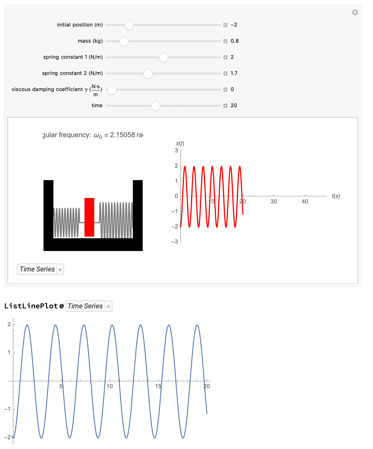
I pulled the code out of the author notebook, figured out where they were make the plot you see, extracted the Plot argument, stuck that inside a table, and added an Iconize so that you can copy the time series out easily:

Manipulate[
 Module[{\[Omega]1, a, b, c, d},
  \[Omega]1 = 1/(2 m) Sqrt[4 m (k1 + k2) - \[Gamma]^2];
  a = Plot[{1.4 Sin[(x1 E^((-\[Gamma] \[Tau])/
              2 m) (Cos[\[Omega]1 \[Tau] + \[Gamma]/(2 m \[Omega]1)
                 Sin[\[Omega]1 \[Tau]]]) + 8) (x - 
           x1 E^((-\[Gamma] \[Tau])/
              2 m) (Cos[\[Omega]1 \[Tau] + \[Gamma]/(2 m \[Omega]1)
                 Sin[\[Omega]1 \[Tau]]]) - \[Pi]) + 2 \[Pi]]}, {x, 
     x1 E^((-\[Gamma] \[Tau])/2 m) ( 
        Cos[\[Omega]1 \[Tau] + \[Gamma]/(2 m \[Omega]1)
            Sin[\[Omega]1 \[Tau]]]) + \[Pi], 4 \[Pi]}, 
    PlotLabel -> 
     Column[{Row[{"angular frequency:", , 
         "\!\(\*SubscriptBox[\(\[Omega]\), \(0\)]\) = ", N[Sqrt[(k1 + k2)/m]], 
         " rad/s"}]}], ImageSize -> {275, 250}, PlotStyle -> {Gray, Thick}, 
    PlotRange -> {{-5 \[Pi], 5 \[Pi]}, {-2, 5}}, Axes -> None, AspectRatio -> 1];
  b = Plot[{Sin[(x1 E^((-\[Gamma] \[Tau])/
             2 m) (Cos[\[Omega]1 \[Tau] + \[Gamma]/(2 m \[Omega]1)
                Sin[\[Omega]1 \[Tau]]]) - 6) (x - 
          x1 E^((-\[Gamma] \[Tau])/
             
             2 m) (Cos[\[Omega]1 \[Tau] + \[Gamma]/(2 m \[Omega]1)
                Sin[\[Omega]1 \[Tau]]]) + \[Pi]) + 2 \[Pi]]}, {x, -4 \[Pi], 
     x1 E^((-\[Gamma] \[Tau])/
         2 m) (Cos[\[Omega]1 \[Tau] + \[Gamma]/(2 m \[Omega]1)
            Sin[\[Omega]1 \[Tau]]]) - \[Pi]}, ImageSize -> {275, 250}, 
    PlotStyle -> {Gray, Thick}];
  c = Show[a, b];
  d = Plot[
    x1 E^((-\[Gamma] tt)/
       2 m) (Cos[\[Omega]1 tt + \[Gamma]/(2 m \[Omega]1)
          Sin[\[Omega]1 tt]]), {tt, -0.1, \[Tau]}, PlotStyle -> {Red, Thick}, 
    AxesLabel -> {t[s], x[t]}, PlotRange -> {{0, 15 \[Pi]}, {-3, 3}}];
  Column[{
    GraphicsRow[{Show[c,
       Graphics[{
         {Thick, Gray,
          Line[{{x1 E^((-\[Gamma] \[Tau])/
                 2 m) (Cos[\[Omega]1 \[Tau] + \[Gamma]/(2 m \[Omega]1)
                    Sin[\[Omega]1 \[Tau]]]) - \[Pi], 
             0}, {x1 E^((-\[Gamma] \[Tau])/
                 2 m) (Cos[\[Omega]1 \[Tau] + \[Gamma]/(2 m \[Omega]1)
                    Sin[\[Omega]1 \[Tau]]]) + \[Pi], 0}}]}, {Red, 
          Rectangle[{x1 E^((-\[Gamma] \[Tau])/
                2 m) (Cos[\[Omega]1 \[Tau] + \[Gamma]/(2 m \[Omega]1)
                   Sin[\[Omega]1 \[Tau]]]) - 
             1.5, -1}, {x1 E^((-\[Gamma] \[Tau])/
                2 m) (Cos[\[Omega]1 \[Tau] + \[Gamma]/(2 m \[Omega]1)
                   Sin[\[Omega]1 \[Tau]]]) + 1.5, 1.5 + m/4}]}, {Black, 
          Polygon[{{-4 \[Pi], -1.1}, {-4 \[Pi], 3}, {-5 \[Pi], 
             3}, {-5 \[Pi], -2}, {5 \[Pi], -2}, {5 \[Pi], 3}, {4 \[Pi], 
             3}, {4 \[Pi], -1.1}, {-4 \[Pi], -1.1}}]}}]], d}],
    Iconize[
     Table[
      {tt, 
       x1 E^((-\[Gamma] tt)/
          2 m) (Cos[\[Omega]1 tt + \[Gamma]/(2 m \[Omega]1) Sin[\[Omega]1 tt]])},
      {tt, -0.1, \[Tau], .001}
      ],
     "Time Series"
     ]
    }]
  ],
 {{x1, -2, "initial position (m)"}, -3, 3, Appearance -> "Labeled"},
 {{m, .8, "mass (kg)"}, 0.5, 3, Appearance -> "Labeled"},
 {{k1, 2, "spring constant 1 (N/m)"}, 1, 3, 
  Appearance -> "Labeled"}, {{k2, 1.7, "spring constant 2 (N/m)"}, 1, 3, 
  Appearance -> "Labeled"}, {{\[Gamma], 0, 
   "viscous damping coefficient \[Gamma] (\!\(\*FractionBox[\(N\[CenterDot]s\), \
\(m\)]\))"}, 0, 1, Appearance -> "Labeled"}, {{\[Tau], 20, "time"}, 0, 15 \[Pi],
   Appearance -> "Labeled"}, ControlPlacement -> Top
 ]

enter image description here

$\endgroup$
7
  • $\begingroup$ I am looking through it. I think that is what I am looking for. I did try to write that equation we were plotting inside the Cases function but it didn't work for some reason. Now, I am not familiar with the TimeSeries function. When I click on it I can just see part of the values. How can I export this as a file? $\endgroup$
    – usernew
    Commented Mar 5, 2021 at 2:21
  • $\begingroup$ Use Export on the dataset as usual $\endgroup$
    – b3m2a1
    Commented Mar 5, 2021 at 5:44
  • $\begingroup$ Do you know why the text file I get has the time and corresponding x values inside brackets and it doesn't look like the example I referred to. In other words, how can I cleanly export this without the brackets and commas so that i can export to excel afterwards. $\endgroup$
    – usernew
    Commented Mar 9, 2021 at 0:45
  • $\begingroup$ @usernew you're gonna have to give me more to go off of than that...did you try Export["your/path/to/file.csv", thatTimeSeries]? $\endgroup$
    – b3m2a1
    Commented Mar 9, 2021 at 0:47
  • $\begingroup$ Ok, I will edit my question to show exactly what I mean. Thank you. $\endgroup$
    – usernew
    Commented Mar 9, 2021 at 0:48

Your Answer

By clicking “Post Your Answer”, you agree to our terms of service and acknowledge you have read our privacy policy.

Not the answer you're looking for? Browse other questions tagged or ask your own question.