3
$\begingroup$

I'm looking for an efficient way to construct a sinc interpolation i.e. an interpolating function of a list of numbers in the form of a Fourier series with a chosen maximum frequency. The input list is supposed to be an equidistant sample of some real smooth function (e.g. a function with a finite-support Fourier transform) and the interpolation should be a continuous function that is a sum of harmonic functions (cosine and sine functions) such that their coefficients are equal to the Fourier coefficients of the list for all frequencies up to the chosen max frequency, (see Wikipedia: Whittaker–Shannon interpolation formula). Increasing the max frequency beyond the band-limit of the original function should give a perfect reconstruction of it. I'd guess there is a predefined Mathematica function doing that but I couldn't find it.

One way would be to apply Interpolation on the list, then NFourierSeries on the resulting InterpolationFunction (choosing the desired max frequency), but this is obviously very inefficient. LowpassFilter should be doing something similar but the output is a list, not a function. One option for an efficient solution that I'm trying to implement is to compute the Fourier coefficients from the list using Fourier, construct a function that is a list of harmonic functions with the right frequencies (e.g. Table[Sin[2 Pi n #/T], {n, nmax}] & for sines) and then Dot-multiply the two lists. I found this excellent post that computes the correct factors: Numerical Fourier transform of a complicated function

$\endgroup$
6
  • 2
    $\begingroup$ Have you seen this and this? $\endgroup$ Commented Jan 10, 2021 at 2:07
  • 1
    $\begingroup$ Maybe this, too. $\endgroup$
    – Michael E2
    Commented Jan 10, 2021 at 3:12
  • $\begingroup$ @J.M.'sennui Thanks! I had seen the second one but not the first. However, these approaches wouldn't be as efficient as I need, for example they use Sum which is slow for large lists. $\endgroup$
    – spyros
    Commented Jan 10, 2021 at 12:06
  • 4
    $\begingroup$ Sinc interpolation is interpolation using the assumption that the spectrum of the function is zero above the sampling rate of the function. So if you sinc-interpolate, then do NFourierSeries, you should find that all the additional terms are zero. An efficient way of doing sinc-interpolation is to Fourier transform, zero-pad the spectrum, then inverse Fourier transform. $\endgroup$
    – mikado
    Commented Jan 10, 2021 at 13:03
  • $\begingroup$ @MichaelE2 Thanks! I should read this more carefully. It seems to go a bit deeper into the efficiency aspect. It should also be possible to make it run faster using Compile. $\endgroup$
    – spyros
    Commented Jan 10, 2021 at 19:27

2 Answers 2

4
$\begingroup$

A Sinc interpolation can be done along the same same idea as a Lagrange interpolation: Assuming we have equally spaced data points, we seek a function ipol that is 1 at x==0 and zero at every other data argument. The sum of ipol[x-x[[i]]] dat[[i]] over i gives then an interpolation function. By this the highest frequency is given by half the sample rate.

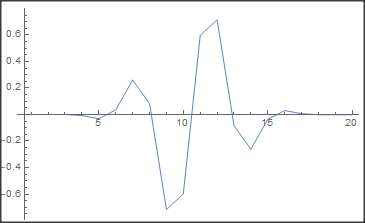
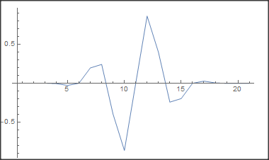
To demonstrate a Sinc interpolation, we first need some arbitrary test data, assuming for simplicity, that the x values are 1,2,..:

n = 20;
dat = Table[Exp[-x^2] Sin[ 4 x], {x, -Pi, Pi, 2 Pi/n}];
ListLinePlot[dat, PlotRange -> All]

enter image description here

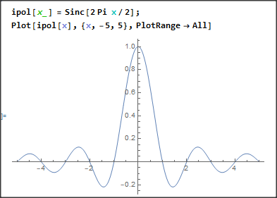
Then we define a scaled Sinc that is 1 at x==0 and zero at every other integer value:

ipol[x_] = Sinc[2 Pi  x/2];
Plot[ipol[x], {x, -5, 5}, PlotRange -> All]

enter image description here

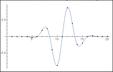
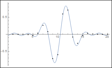
Now, we place such an function at every data point and multiply it with the value of the data point. Then we plot it together with the original data points :

fun[x_] = Table[ipol[x - y], {y, Length[dat]}].dat;
Plot[fun[x], {x, 0, 20}, PlotRange -> All, 
 Epilog -> Point[Transpose@{Range[n + 1], dat}]]

enter image description here

$\endgroup$
8
  • $\begingroup$ Sinc[2 Pi x/2] is just Sinc[Pi x], no? $\endgroup$ Commented Jan 10, 2021 at 11:24
  • $\begingroup$ Thanks! I need to apply this operation on ~10000 lists of length ~1000 each, which is why I need an efficient implementation, but this simple solution may actually be sufficient for my purposes. I would first apply a LowpassFilter on each list with a reasonable max frequency and then construct the function list Table[ipol[x - y], {y, Length[dat]}] only once and Dot-multiply it with each of the filtered lists. $\endgroup$
    – spyros
    Commented Jan 10, 2021 at 14:03
  • $\begingroup$ For some reasons, I would still prefer it if the output was a Fourier series instead of a sum of sinc-functions (for example I would like to be able to construct periodic interpolations as with the option Padding -> "Periodic" of Interpolation, which would be simpler using sines and cosines). But of course your solution gives the true sinc-interpolation, the truncated Fourier series is not precisely the same and it's not a true interpolation either. $\endgroup$
    – spyros
    Commented Jan 10, 2021 at 14:04
  • 1
    $\begingroup$ @Daniel Lichtblau. Hi Daniel, I think if you truncate the Fourier transform, the resulting back transform goes no more through the original points. You will then have a smoothing operation and no interpolation. $\endgroup$ Commented Jan 10, 2021 at 20:56
  • 1
    $\begingroup$ @DanielHuber Actually my post wasn't so clear on this: I'm interested in both the smoothing operation and the interpolation as a special case (when the number of frequencies kept is equal to the size of the original list). $\endgroup$
    – spyros
    Commented Jan 11, 2021 at 0:05
3
$\begingroup$

If we want to use FFT to get an expansion in circular functions we can proceed as follows:

FFT can be look at as a base change with the new base functions: Exp[2Pi I x f]. This is not too simple, because the FFT returns the coefficients like: First DC component, then coefficients of functions with increasing frequencies and pos. exponents. Up to the highest frequency (there may be one or two). Then down again in frequency with negative exponents.

Again we need same test data:

n = 20;
dat = Table[Exp[-x^2] Sin[4 x], {x, -Pi, Pi, 2 Pi/(n - 1)}];
ListLinePlot[dat, PlotRange -> All]

![enter image description here

Then we calculate the FFT and if we want to smooth, truncate it:

fft = Fourier[dat];
smooth = 0;
If[smooth > 0, 
  If[EvenQ[n], fft[[2 + n/2 - smooth ;; n/2 + smooth]] = 0, 
   fft[[(n + 1)/2 - smooth ;; (n + 1)/2 + smooth]] = 0]];

We now have the coefficients of the new base and can assemble the searched for function and plot the result:

(*fourier synthese*)
tab = Table[
   Exp[ -2 Pi I If[i < (n + 1)/2, (i - 1), -(n + 1 - i)] (x - 1)/
      n], {i, n}] ;
fun[x_] = (tab.fft + 
     If[EvenQ[n], 
      fft[[1 + n/2]] (E^(-I \[Pi] (-1 + x)) - E^(I \[Pi] (-1 + x)))/2,
       0])/Sqrt[n];
Plot[fun[x], {x, 0, n}, PlotRange -> All, 
 Epilog -> Point[Transpose[{Range[n], dat}]]]

No truncation:

enter image description here

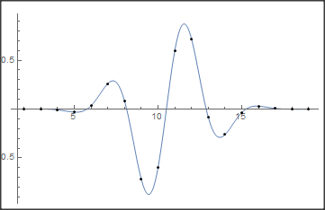
With truncation (smooth=4):

enter image description here

As you see, truncation is not without drawbacks, it increases the wiggles. This is because use a rectangular window in the frequency domain. To improve, we would use a smoother window like Hamming, von Hann, ...

The function fun is now in exponential form. If you want it expanded in sin and cos:

fun[x_] = fun[x] // ComplexExpand // Chop
$\endgroup$

Your Answer

By clicking “Post Your Answer”, you agree to our terms of service and acknowledge you have read our privacy policy.

Not the answer you're looking for? Browse other questions tagged or ask your own question.