3
$\begingroup$

How to overcome this error?

ode = D[theta[x], {x, 2}] == SH*theta[x]^2
sol = ParametricNDSolveValue[{ode, theta[0] == 1, theta'[1] == 0}, theta[x], {x, 0, 1}, {SH}]
Ns[SH_, Tr_] := SH*sol[SH]*(Log[1 + Tr*sol[SH]] - sol[SH]/(sol[SH] + (Tr - 1)^(-1)))
Plot[Ns[10, 1.2], {x, 0, 1}]

ParametricNDSolveValue::ndsz: At x$2319 == 0.940612307913943`, step size is effectively zero; singularity or stiff system suspected.

$\endgroup$
1
  • $\begingroup$ Notice also that at least the differential equation solution works fine for other values of SH. For instance, sol[3] works fine, and so therefore does Ns[3, 1.2] for instance. $\endgroup$
    – MarcoB
    Commented Jan 6, 2021 at 3:14

2 Answers 2

4
$\begingroup$

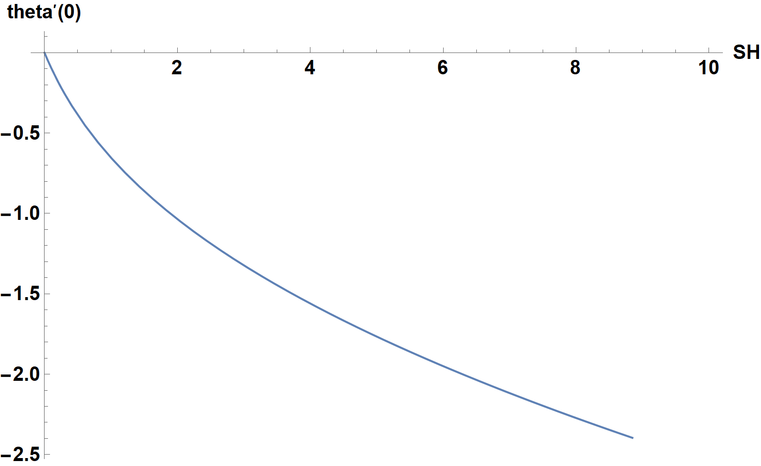
ParametricNDSolve by default using the "Shooting" method with some simple initial-value guess when solving boundary-value problems, such as this. Sometimes, that initial-value guess leads to the error cited in the Question. If so, providing a better initial guess is required. To obtain one in this case, first computer the value of theta'[0] that solves the ODE as a function of SH.

soltst = ParametricNDSolveValue[{ode, theta[0] == 1, theta'[1] == 0}, theta'[0], 
    {x, 0, 1}, {SH}];
Plot[soltst[sh], {sh, 0, 10}, ImageSize -> Large, AxesLabel -> {SH, theta'[0]}, 
    LabelStyle -> {15, Bold, Black}]

enter image description here

We see that the computation with the default value of an initial guess for theta'[0] (probably zero), fails at about SH = 8.9 but, more importantly, that the true value of theta'[0] becomes progressively less than zero. Use this insight as follows:

sol = ParametricNDSolveValue[{ode, theta[0] == 1, theta'[1] == 0}, theta[x], {x, 0, 1}, 
    {SH}, Method -> {"Shooting", "StartingInitialConditions" -> 
    {theta'[0] == -.8 Sqrt[SH]}}]

which yields

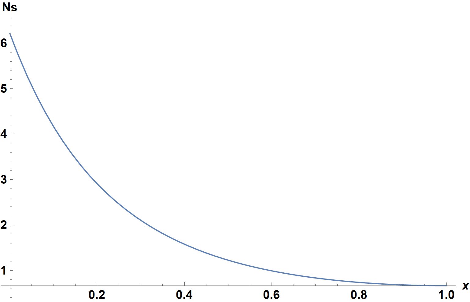
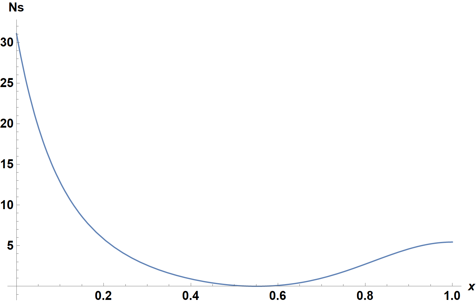
Plot[Ns[10, 1.2], {x, 0, 1}, ImageSize -> Large, AxesLabel -> {x, Ns}, 
    LabelStyle -> {15, Bold, Black}]

![enter image description here

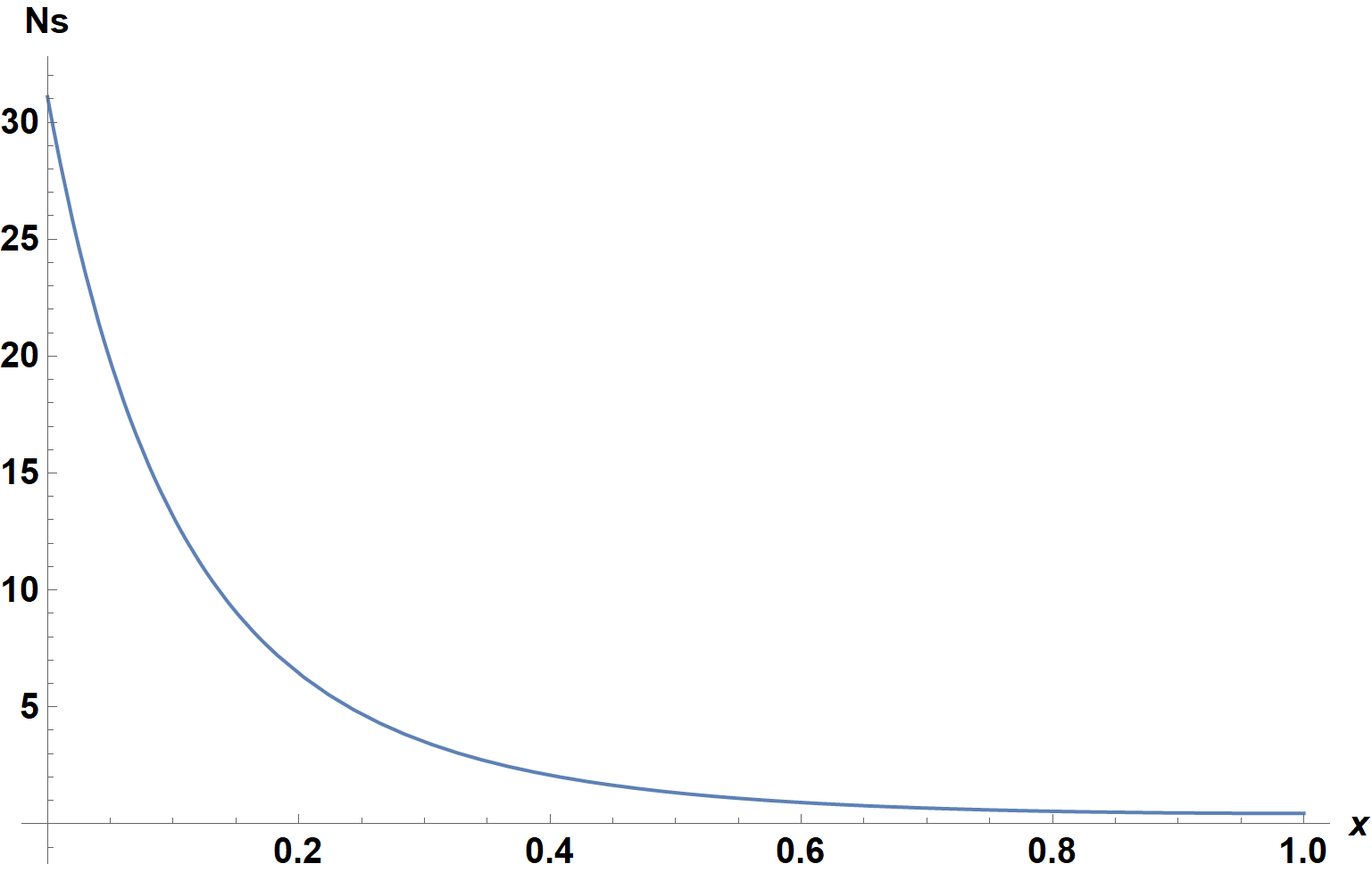
as desired. Note that this initial guess for theta'[0] works up to about SH = 60, after which a more refined initial guess is needed. In a comment, the OP also requested a result for SH = 50

![enter image description here

Addendum: Second Solution

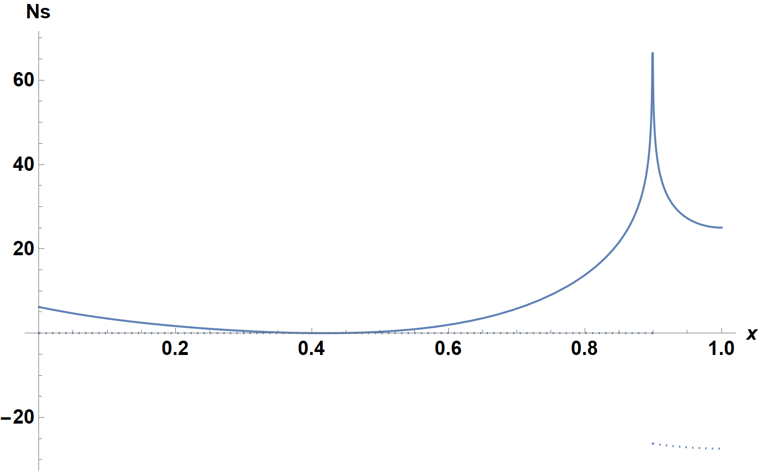
I discovered by accident that a second solution exists. Redefine sol to use as an initial guess, theta'[0] == -3.3 - .05 SH. Then, the result for SH = 10(obtained using ReImPlot) is

![enter image description here

Note that it is singular at about x = 0.9, although not due to a singularity in sol[10] but rather to the choice of Tr = 1.2. For SH = 50, the result is

![![enter image description here

I do not believe that there are additional continuous solutions.

$\endgroup$
6
  • $\begingroup$ How to obtained an initial guess for SH=50? $\endgroup$
    – zhk
    Commented Jan 7, 2021 at 0:32
  • $\begingroup$ Would you settle for a symbolic solution, on which I now am working? $\endgroup$
    – bbgodfrey
    Commented Jan 7, 2021 at 0:37
  • $\begingroup$ Yes of course but I would like to learn how to find the correct initial condition. $\endgroup$
    – zhk
    Commented Jan 7, 2021 at 0:37
  • $\begingroup$ As requested, I have provided an improved initial guess and a solution for SH= 50. However, the constraints on the initial guess become more and more severe as SH is increased, and progressively more work is needed to find a suitable expression. $\endgroup$
    – bbgodfrey
    Commented Jan 7, 2021 at 2:23
  • $\begingroup$ Thanks for your efforts. But my question, how you find theta'[0] == -.8 Sqrt[SH]? $\endgroup$
    – zhk
    Commented Jan 7, 2021 at 2:25
2
$\begingroup$

Another way is to solve the ODE exactly and use FindRoot to solve for the boundary conditions. There are infinitely many solutions for the parameters C[1] and C[2], but they yield only two distinct solutions, one of which has a singularity.

Clear[Ns, sol, dsol, findparam];
ode = D[theta[x], {x, 2}] == SH*theta[x]^2;
bcs = {theta[0] == 1, theta'[1] == 0};
dsol[SH_] = DSolveValue[{ode}, theta, {x, 0, 1}];
findparam[SH_?NumericQ, c1_?NumericQ, c2_?NumericQ] := 
  FindRoot[bcs /. theta -> dsol[SH] /. 
     Thread[{C[1], C[2]} -> {u, v}], {{u, c1}, {v, c2}}, 
    WorkingPrecision -> (Precision@{SH, c1, c2} /. 
       p_?(! NumericQ[#] &) :> MachinePrecision)] /. 
   Thread[{u, v} -> {C[1], C[2]}];
sol[SH_, c1_?NumericQ, c2_?NumericQ] := 
  theta[x] /. theta -> dsol[SH] /. {C[1] -> c1, C[2] -> c2};
Ns[SH_, Tr_, c1_?NumericQ, c2_?NumericQ] := With[{s = sol[SH, c1, c2]},
   SH*s*(Log[1 + Tr*s] - s/(s + (Tr - 1)^(-1)))
   ];
Plot[
 Evaluate[Ns[10, 1.2`44, C[1], C[2]] /. findparam[10, 1, 1/2]]
 , {x, 0, 1}]

I used ContourPlot initially to see where the BCs might be satisfied, but the following is more accurate once you know where to look:

ics = {theta[0], theta'[0]}; negsol = 
 Table[Quiet@Check[findparam[10, k, -5.`32], $Failed], {k, 5}];
possol = Table[Quiet@Check[findparam[10, k, 0.1`32], $Failed], {k, 5}];
paramsols = 
 DeleteDuplicates[Join[negsol, possol] /. $Failed -> Nothing, 
  Norm[(ics /. theta -> dsol[10] /. #1) - (ics /. 
         theta -> dsol[10] /. #2)] < 10^-8 &]
(*
{{C[1] -> 0.74517523946507200325661614980780, 
  C[2] -> -4.4126787665722546011617781190585},
 {C[1] -> 11.430806610070804819523668005587, 
  C[2] -> 0.14721944767874966824783455933860}}
*)

ReImPlot[
 Evaluate[{1, 10} (Ns[10, 1.2`44, C[1], C[2]] /. paramsols)],
 {x, 0, 1},
 WorkingPrecision -> 16, PlotRange -> All, 
 Method -> {"BoundaryOffset" -> False},
 Frame -> True, 
 FrameTicks -> {{Automatic, Charting`ScaledTicks[{10 # &, #/10 &}]}, 
   Automatic}]
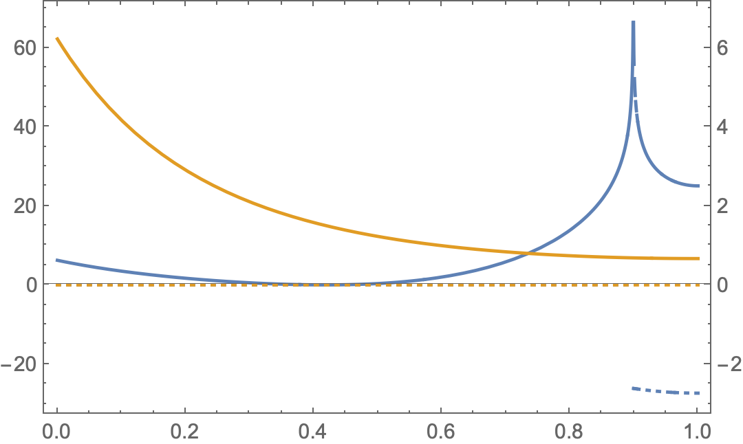
$\endgroup$

Your Answer

By clicking “Post Your Answer”, you agree to our terms of service and acknowledge you have read our privacy policy.

Not the answer you're looking for? Browse other questions tagged or ask your own question.