1
$\begingroup$

I'm trying to extract the distribution parameters of the sub-distributions which comprise a mixed normal distribution.

I'll give my attempts so far.

First the simulated data:

MixedGaussiaData = Apply[Join, {RandomVariate[NormalDistribution[0, 2], 300], RandomVariate[NormalDistribution[0, 0.7], 500], RandomVariate[NormalDistribution[0, 0.4], 500], RandomVariate[NormalDistribution[0, 1], 200]}];

Which when plotted looks like this:

enter image description here

So we have four normal distributions with different $\sigma$ values and different number of points, but all distributions have a common mean value $\mu = 0$.

I define my $n$ mixed-normal distribution as:

NMixedGaussian[n_] := MixtureDistribution[Array[w, n], MapThread[NormalDistribution[#1, #2] &, {Array[m, n], Array[s, n]}]]

Then using FindDistributionParameters

FourMixedNormalMLE = FindDistributionParameters[MixedGaussiaData, NMixedGaussian[4], ParameterEstimator->{"MaximumLikelihood", PrecisionGoal->1, AccuracyGoal->1}]

If I plot the result, it looks pretty good:

enter image description here

However if we take a look at the results, they're not that good when compared to the inputs of the simulation:

mMLE = Array[m, 4] /. FourMixedNormalMLE
sMLE = Array[s, 4] /. FourMixedNormalMLE
wMLE = Array[w, 4] /. FourMixedNormalMLE

{0.0284676, 0.00902554, 0.0930328, -0.470579}
{1.8648, 0.274301, 0.667947, 0.385259}
{0.237727, 0.192302, 0.475281, 0.0946906}

Second attempt:

I tried explicitly defining the Mixed-Gaussain function with ProbabilityDensity:

Clear[w, m, s, n];
NMixedGaussian[n_] := MixtureDistribution[Array[w, n], MapThread[NormalDistribution[#1, #2] &, {Array[m, n], Array[s, n]}]]

NMixGauss = NMixedGaussian[4];
NMixGaussPDF[z_] = FullSimplify[PDF[NMixGauss, z], DistributionParameterAssumptions[NMixGauss]]

NMixGaussPD = ProbabilityDistribution[NMixGaussPDF[z], {z, -Infinity, Infinity}, Assumptions -> DistributionParameterAssumptions[NMixGauss]]

FourMixedNormalPDFMLE = FindDistributionParameters[MixedGaussiaData, NMixGaussPD, ParameterEstimator->{"MaximumLikelihood", PrecisionGoal->1, AccuracyGoal->1}]

This makes it worse. I think the main issue might be initial values and constraints, but I'm not sure how to best implement this. Does anyone have any suggestions?

One thing I noticed is that the weights produced by FindDistributionParameters don't seem to make sense. They sum to one, but none seem to correspond to weights defined by $1/\sigma^{2}$ or $1/\sigma_{\rm{SE}}^{2}$


Addition: What I'm trying to achieve is another way of performing a weighted mean. I could divide the simulated data up into chunks/bins, find the $\mu$ and $\sigma$ for each one and perform a weighted mean. I want to avoid binning if possible, hence this approach.

Just to be a bit more explicit in what I am trying to do/expect to see. Here I've just performed a simple weighted average and determined the associated standard error:

SeedRandom[1]

Gaussian1 = RandomVariate[NormalDistribution[0, 2], 300];
Gaussian2 = RandomVariate[NormalDistribution[0, 0.7], 500];
Gaussian3 = RandomVariate[NormalDistribution[0, 0.4], 500];
Gaussian4 = RandomVariate[NormalDistribution[0, 1], 200];

M = {Mean[Gaussian1], Mean[Gaussian2], Mean[Gaussian3], Mean[Gaussian4]};
S = {StandardDeviation[Gaussian1], StandardDeviation[Gaussian2], StandardDeviation[Gaussian3], StandardDeviation[Gaussian4]};
SE = {StandardDeviation[Gaussian1]/Sqrt[Length[Gaussian1]], StandardDeviation[Gaussian2]/Sqrt[Length[Gaussian2]], StandardDeviation[Gaussian3]/Sqrt[Length[Gaussian3]], StandardDeviation[Gaussian4]/Sqrt[Length[Gaussian4]]};
W = 1 / SE^2;

Around[WU = Total[W M]/Total[W], WSE = Sqrt[(Total[W M^2]/Total[W] - (Total[W M]/Total[W])^2 Length[W]/(Length[W] - 1))  / Length[W]]]

OUT = Around[-0.010808335694884515`, 0.0184845352965455]


mMLE = Array[m, 4] /. FourMixedNormalMLE
sMLE = Array[s, 4] /. FourMixedNormalMLE
wMLE = Array[w, 4] /. FourMixedNormalMLE

Around[WUMLE = Total[wMLE mMLE], WSEMLE = Sqrt[(Total[wMLE mMLE^2] - (Total[wMLE mMLE])^2 Length[wMLE]/(Length[wMLE] - 1))  / Length[wMLE]]]

OUT = Around[0.008160465141904528, 0.07937540663098669]

If I compare the results from those determined from a weighted mean, to those I get from FindDistributionParameters they are quite different.

$\endgroup$
15
  • 1
    $\begingroup$ Something like: skd = SmoothKernelDistribution[data]; {weights, means, bandwidth} = skd[[2]]; Show[Histogram[data, Automatic, "PDF"], Plot[PDF[skd, x], {x, -3, 3}, PlotStyle -> Thick]] then you have Mean[WeightedData[means, weights]] which coincides with Mean[data] anyway. Also it has an option like MaxMixtureKernels -> 50 so you can limit the number of mixture distributions, but don't set this too low or it starts to misrepresent the data. $\endgroup$
    – flinty
    Commented Nov 9, 2020 at 21:02
  • 1
    $\begingroup$ A minor point: your data is not from a mixture distribution in the sense that while the weights are constant, the actual realization of counts from each subpopulation is not. To get a sample from the mixture distribution you're trying to fit consider: parms = {Thread[Array[w, 4] -> {300, 500, 500, 200}], Thread[Array[m, 4] -> {0, 0, 0, 0}], Thread[Array[s, 4] -> {2, 0.7, 0.4, 1}]} // Flatten; data = RandomVariate[NMixedGaussian[4] /. parms, 1500]. $\endgroup$
    – JimB
    Commented Nov 9, 2020 at 21:14
  • 2
    $\begingroup$ "One thing I noticed is that the weights produced by FindDistributionParameters don't seem to make sense. They sum to one, but none seem to correspond to weights 1/sigma^2" I don't understand this remark. Why should the weights have anything to do with the standard deviation? $\endgroup$ Commented Nov 9, 2020 at 21:38
  • 2
    $\begingroup$ Note that there's no reason to expect that the order in which you constructed the data will necessarily match to the order in which the estimates of the parameters are returned. $\endgroup$
    – JimB
    Commented Nov 9, 2020 at 22:25
  • 1
    $\begingroup$ It's the collection of the 4 triplets of parameters that matter but the 4 triplets returned might occur in any order. I'm not talking about the order of the data points. I'm writing up an answer as we speak. $\endgroup$
    – JimB
    Commented Nov 10, 2020 at 3:42

2 Answers 2

1
$\begingroup$

We had a discussion and we came to the conclusion (I think) that what was needed was a "mixed model" rather than a "mixture model". A simplified definition of a mixed model is a regression with more than one error term (resulting in some observations being correlated with other observations). Mathematica does not currently offer a direct way to analyze mixed models but certainly has the basic tools to do so.

For this particular question the mixed model can written as follows:

$$y_{ij}=\mu+\gamma_i+\epsilon_{ij}$$

where $y_{ij}$ is the $j$-th observation of subpopulation $i$, $\mu$ is the overall mean, $\gamma_i \sim N(0,\sigma_P^2)$ is a random effect of subpopulation $i$, and $\epsilon_{ij} \sim N(0,\sigma_i^2)$ is the measurement error for each of the $n_i$ observations from subpopulation $i$. All random variables are assumed to be independent of each other.

The objective is to estimate $\mu$ (and get an appropriate measure of precision).

First, generate some data in Mathematica.

μ = 2 ;(* Overall mean *)
σPop = 0.1; (* Standard deviation of subpopulation deviations from μ *)

σ = {0.2, 0.2, 0.4, 0.4, 0.7, 1, 1, 1, 2, 2}; (* Subpopulation standard deviations *)
n = {100, 200, 100, 100, 300, 400, 50, 50, 25, 50}; (* Subpopulation sample sizes *)

(* Subpopulation deviations from μ *)
SeedRandom[12345];
deviations = RandomVariate[NormalDistribution[0, σPop], 10];

(* Put together subpopulation identification and associated observations *)
data = Flatten[Table[Table[{j, μ + deviations[[j]] + 
       RandomVariate[NormalDistribution[0, σ[[j]]]]},
     {i, n[[j]]}], {j, 10}], 1];

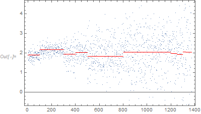
A plot of the data and the random deviations for each subpopulation:

a = Accumulate[n];
levels = Table[If[i == 1, {{1, μ + deviations[[i]]}, {a[[1]], μ + deviations[[i]]}},
    If[i == 10, {{a[[i - 1]] + 1, μ + deviations[[i]]}, {a[[10]], μ + deviations[[i]]}},
     {{a[[i - 1]] + 1, μ + deviations[[i]]}, {a[[i]], μ + deviations[[i]]}}]], {i, 10}];
Show[ListPlot[data[[All, 2]], Frame -> True], 
 ListPlot[levels, Joined -> True, PlotStyle -> Red]]

Data and deviations from mean

One can use RLink to estimate all of the parameters. For now I just show how to get the estimate of the overall mean (appropriately weighted) and an associated standard error. First get RLink working.

Needs["RLink`"]
RLinkResourcesInstall[]
InstallR["RHomeLocation" -> "c:/Program Files/R/R-3.6.1"]

Now for the analysis with the previously created data.

RSet["y", data[[All, 2]]];
RSet["pop", data[[All, 1]]];
result = REvaluate["{
    # Create a data frame with the measurement and associated subpopulation;
    d=data.frame(y=y, pop=factor(pop));
    # Load the nlme library;
    library(nlme);
    # Run analysis;
    results=lme(y ~ 1, data=d, random = ~ 1|pop, 
      weights=varIdent(form=~1|pop),
      control=lmeControl(maxIter = 500, msMaxIter = 500));
    
    # Return the " weighted mean " and a standard error;
    summary(results)$tTable
    }"];
(* Make the result look nice *)
TableForm[result[[1]], TableHeadings -> result[[2, 1, 2]]]

Result from fitting a linear mixed model

If there is variability in the means of the subpopulations, then this technique will generally have a much smaller standard error for the mean than using a standard weighted mean. The main reason for that is that the standard weighted mean (described by the OP) assumes that the means of the subpopulations are all essentially identical. When the subpopulation means are not identical, then the precision is adversely affected.

So a "mixture model" is a random mixture of different distributions and you don't know which observation comes from any particular distribution. But you can still estimate all of the parameters knowing the number (and type) of distributions involved.

A "mixed model" is where you known which subpopulation is associated with each observation and it assumes that the deviation of the subpopulation mean follows a some distribution (usually one assumes normality but that is not required).

$\endgroup$
0
1
$\begingroup$

While the estimation process will process any dataset and real datasets never really match the what the model expects, the dataset you created isn't a mixture distribution in the usual sense in that you have the counts of each subpopulation fixed. In a standard mixture distribution, the counts of each subpopulation will vary.

To generate data for your mixture models I recommend something like the following:

NMixedGaussian[n_] := MixtureDistribution[Array[w, n], 
  MapThread[NormalDistribution[#1, #2] &, {Array[m, n], Array[s, n]}]]
parms = {Thread[Array[w, 4] -> {300, 500, 500, 200}/1500],
    Thread[Array[m, 4] -> {0, 0, 0, 0}],
    Thread[Array[s, 4] -> {2, 0.7, 0.4, 1}]} // Flatten;
SeedRandom[12345];
data = RandomVariate[NMixedGaussian[4] /. parms, 1500];

You used FindDistributionParameters which works fine but its drawback is that you just get estimates and no measures of precision or correlation among parameter estimators. I use FindDistributionParameters just to get starting values for a relatively simple set of steps that gets you the measures of precision. With those measures you can see if the precision levels explain any differences you see from the "true" parameters. (And it's even more helpful when you just have the data and not the "true" parameters that generated the data.)

Here is a brute force approach:

(* FindDistributionParameters *)
FourMixedNormalMLE = FindDistributionParameters[data, NMixedGaussian[4],
  ParameterEstimator -> {"MaximumLikelihood", PrecisionGoal -> 10,
    AccuracyGoal -> 10, MaxIterations -> 5000}]
(* {w[1] -> 0.189239, w[2] -> 0.504157, w[3] -> 0.187723, w[4] -> 0.118881, 
    m[1] -> -0.147546, s[1] -> 2.02087, m[2] -> 0.0856405, s[2] -> 0.40548, 
    m[3] -> 0.437306, s[3] -> 0.856352, m[4] -> -0.794093, s[4] -> 0.463292} *)

(* Maximize log likelihood using the previous solution as starting values *)
logL = LogLikelihood[NMixedGaussian[4] /. w[4] -> 1 - w[1] - w[2] - w[3], data];
mle = FindMaximum[{logL, 
   0 < w[1] < 1 && 0 < w[2] < 1 && 0 < w[3] < 1 && w[1] + w[2] + w[3] < 1
    && s[1] > 0 && s[2] > 0 && s[3] > 0 && s[4] > 0},
  Delete[FourMixedNormalMLE /. Rule -> List, 4]]
(* {-2013.26, {w[1] -> 0.18932, w[2] -> 0.50593, w[3] -> 0.192173, 
  m[1] -> -0.14801, m[2] -> 0.0831314, m[3] -> 0.416784, m[4] -> -0.809995, 
  s[1] -> 2.02032, s[2] -> 0.406299, s[3] -> 0.863456, s[4] -> 0.453506}} *)
    
(* Estimate the covariance and correlation matrices *)
cov = -Inverse[(D[logL, {{w[1], w[2], w[3], m[1], m[2], m[3], m[4], s[1], 
  s[2], s[3], s[4]}, 2}]) /. mle[[2]]];
cor = Table[cov[[i, j]]/Sqrt[cov[[i, i]] cov[[j, j]]], {i, 11}, {j, 11}];

(* Standard errors for parameters *)
stdErr = Sqrt[Diagonal[cov]]
(* {0.0451595, 0.215176, 0.343823, 0.172553, 0.176252, 1.46912, 1.09217, 
     0.161291, 0.0847135, 0.51714, 0.673961} *)

So it seems that you want a "parametric" approach to obtain a better estimate the mean of a distribution from a sample knowing that it is a mixture of normals. However, just using the sample mean and the sample standard error seems a lot simpler and might very well have similar precision.

From the estimated parameters an estimate of the mean is

{w[1], w[2], w[3], 1 - w[1] - w[2] - w[3]}.{m[1], m[2], m[3], m[4]} /. mle[[2]]
(* 0.00294456 *)

If you just looked at the sample mean:

Mean[data]
(* 0.00294456 *)

The values are identical. But I'm likely not understanding your objective.

The "true" mean and standard deviation for your example:

#[NMixedGaussian[4] /. parms] & /@ {Mean, StandardDeviation}
(* {0., 1.07238} *)

Mean and standard deviation from the data:

#[data] & /@ {Mean, StandardDeviation}
(* {0.00294456, 1.06693} *)

Mean and standard deviation from the estimated parameters:

#[NMixedGaussian[4] /. w[4] -> 1 - w[1] - w[2] - w[3]] /. mle[[2]] & /@ {Mean, StandardDeviation}
(* {0.00294456, 1.06657} *)

All match up pretty well.

$\endgroup$
10
  • $\begingroup$ Thanks for taking the time to prepare an answer. My confusion arises in that if I split the data up by distribution, and calculate a weighted mean and standard error I get a different answer and different standard error, if you have a look at my latest edit you can see the difference in values. $\endgroup$
    – user27119
    Commented Nov 10, 2020 at 5:51
  • $\begingroup$ Your Around statements have an incorrect formula for the standard deviation because both of those statements don't include appropriate mention of S (the standard deviations of the individual data sets). But if your objective is to look at only the complete data set which does not identify which subpopulation to which a sample belongs, then I don't understand the attempt at using sample estimates of the mean and standard deviations as if the identity of each sample point is know. Clearly, I'm not understanding your "weighted mean" objective. $\endgroup$
    – JimB
    Commented Nov 10, 2020 at 20:50
  • $\begingroup$ They are included via the weights, I define the weights as $W = 1/(S^{2} / n)$. I think this is correct? ${\rm{Var(x)}} = \frac{n}{n-1}\left(\frac{\sum_i w_{i} x^{2}_{i}}{\sum_{i} w_{i}} - (\bar{x})^{2}\right)$ is the formula I use. Could you show me what you think I should be using? $\endgroup$
    – user27119
    Commented Nov 10, 2020 at 21:05
  • $\begingroup$ I see. But the second Around doesn't include any standard deviations. And I'll check the formula you just mentioned. $\endgroup$
    – JimB
    Commented Nov 10, 2020 at 21:41
  • $\begingroup$ Just so it's easier this is where I got the formula from: seismo.berkeley.edu/~kirchner/Toolkits/Toolkit_12.pdf $\endgroup$
    – user27119
    Commented Nov 10, 2020 at 21:54

Your Answer

By clicking “Post Your Answer”, you agree to our terms of service and acknowledge you have read our privacy policy.

Not the answer you're looking for? Browse other questions tagged or ask your own question.