1
$\begingroup$

I tried to get a dynamic plot of the following function using the simple command:

g[x_, y_, z_] := (x^3 y^5 E^(-2*z*n))/(x^2 + y^2)

Manipulate[
  Plot[g[x, y, z], {x, -10, 10}, PlotRange -> Automatic], 
  {n, -7, 7}]

However, I get an empty plot. What went wrong with this command?

$\endgroup$
9
  • 1
    $\begingroup$ Also, you need to specify values for y and z $\endgroup$
    – xzczd
    Commented Sep 24, 2020 at 11:52
  • $\begingroup$ @xzczd I did specify values for y inside the plot function but I still get an empty graph nonetheless. So I tried to simplify the general manipulate command even more and only included x values but got the same output. $\endgroup$
    – Kurapika
    Commented Sep 24, 2020 at 12:00
  • 1
    $\begingroup$ To be more specific, you need to make n explicit with e.g. g[x_, y_, z_, n_] := (x^3 y^5 E^(-2*z*n))/(x^2 + y^2); Manipulate[Plot[g[x, 1, 1, n], {x, -10, 10}, PlotRange -> Automatic], {n, -7, 7}] Please check the linked post for more info. $\endgroup$
    – xzczd
    Commented Sep 24, 2020 at 12:04
  • $\begingroup$ Okay, I see what I missed. Thanks! One thing I'd like to know is that if I wanted to include ranges for y and z as well instead of assuming them inside g[x,y,z,n] could I state them inside the plot function? Is the current command enough to do that or would I have to make changes? $\endgroup$
    – Kurapika
    Commented Sep 24, 2020 at 12:11
  • $\begingroup$ What do you mean by "I wanted to include ranges for y and z as well instead of assuming them inside g[x,y,z,n] could I state them inside the plot function"? $\endgroup$
    – xzczd
    Commented Sep 24, 2020 at 12:16

3 Answers 3

4
$\begingroup$
Clear["Global`*"]

g[x_, y_, z_, n_] := (x^3 y^5 Exp[-2*z*n])/(x^2 + y^2)

Manipulate[
 Module[{x, func, t, var},
  If[plt == 1,
   var = "z"; func = g @@ Rationalize[{x, y, t, n}],
   var = "y"; func = g @@ Rationalize[{x, t, z, n}]];
  Plot3D[func, {x, -10, 10}, {t, -10, 10},
   WorkingPrecision -> 20,
   MaxRecursion -> 5,
   AxesLabel -> (Style[#, 14, Italic, Bold] & /@ {"x", var, "g "}),
   ClippingStyle -> None,
   PlotLabel -> Style[StringForm["g = ``", 
      g["x", "y", "z", "n"]], Italic, 14]]],
 {{n, 0}, -7, 7, 0.2, Appearance -> "Labeled"},
 {{y, 1}, -10, 10, 0.2, Appearance -> "Labeled"},
 {{z, 1}, -10, 10, 0.2, Appearance -> "Labeled"},
 {{plt, 2, "Plot"}, {
   1 -> "Fixed value of y",
   2 -> "Fixed value of z"}},
 LabelStyle -> Medium]

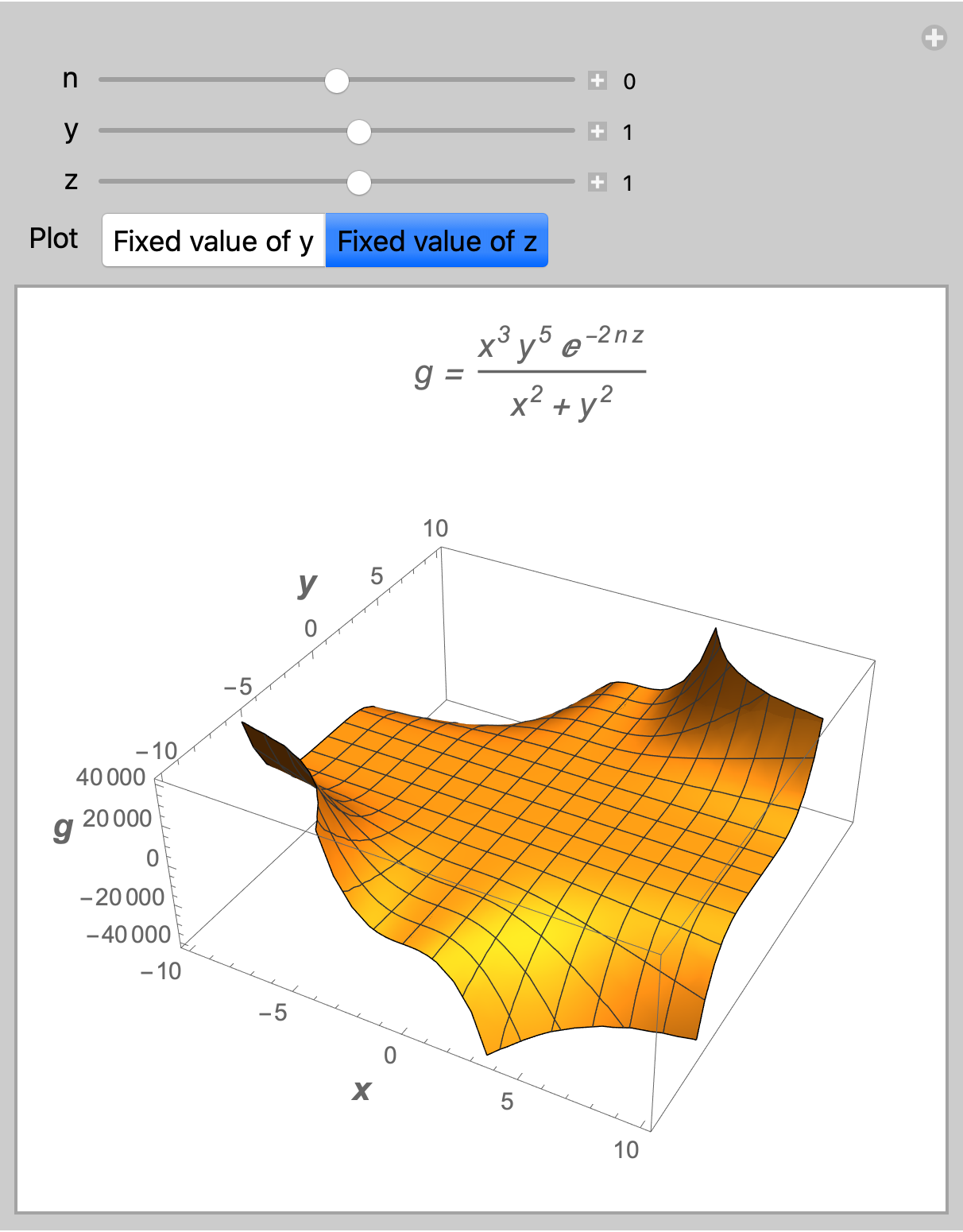
enter image description here

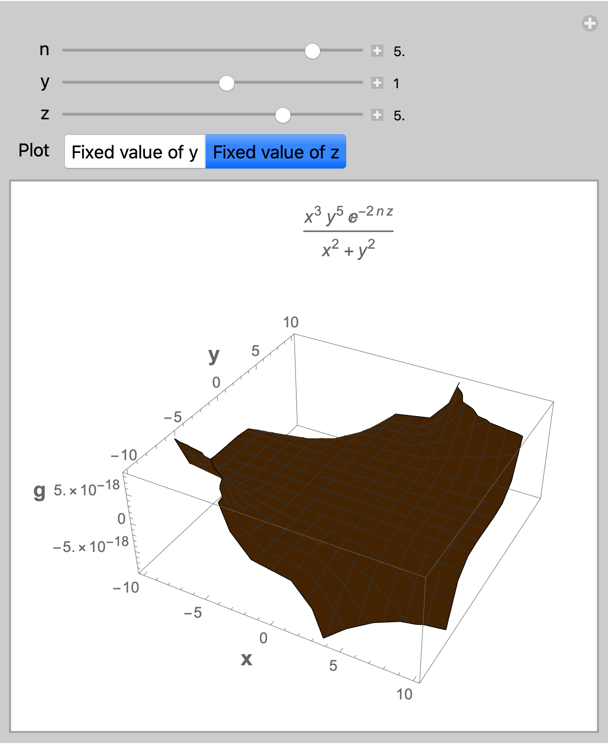
However, note that for fixed values of z and relatively large positive products, n * z, the plot unexpectedly turns dark without any error messages. For example, enter image description here

$\endgroup$
3
$\begingroup$

Maybe use the SliceContourPlot3D to display the level sets of g[x,y,z,n] is easy and faster.

Clear["`*"];
g[x_, y_, z_, n_] := (x^3 y^5 E^(-2*z*n))/(x^2 + y^2);
Manipulate[
 SliceContourPlot3D[
  g[x, y, z, n], {"CenterPlanes"}, {x, -10, 10}, {y, -10, 
   10}, {z, -10, 10}, Contours -> 50, PerformanceGoal -> "Quality", 
  ColorFunction -> "BrightBands", PlotTheme -> "Detailed"], {n, -7, 7,
   1}]

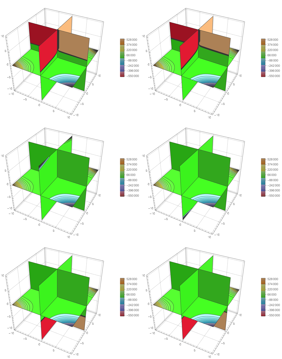
enter image description here

$\endgroup$
0
$\begingroup$

Let us start with reading the question.

The given function is

 (x^3 y^5 E^(-2*z*n))/(x^2 + y^2)

this is dependent on x, y, z and n. So the function has to reflect this four parameters:

g[x_,y_,z_,n_]:=(x^3 y^5 E^(-2*z*n))/(x^2 + y^2)

The polynomial in the denominator has no zeros on the Reals. The multinomial in the nominator has a coefficient functions that dominates in the cases n<0 in the positive first quadrant, for n>0 in the third negative quadrant. So it is not sensible to visualize the plot on these quadrants for AbsReal@x >1 && AbsReal@y >>1.

Whether a net is nicer or contours is a matter of taste.

The first answer causes problems in the plot surface: Plot3D.
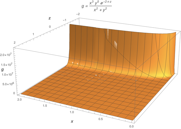
As far as my insight the range {-10,10} addresses this as the main target. Since WorkingPrecision and MaxRecursion do not fix the problem for all parameter combinations the maximum limits are necessary. The borders of the surface can even get very rugged for {0,2}x{0,2}.

Such a realization looks smooth and allows insight:

Manipulate[
 Module[{x, func, t, var}, 
  If[plt == 1, var = "z"; func = g @@ Rationalize[{x, y, t, n}], 
   var = "y"; func = g @@ Rationalize[{x, t, z, n}]];
  Plot3D[Table[func /. n -> m, {m, -4, 4, 2}], {x, -1, 1}, {t, -1, 1},
    WorkingPrecision -> 20, MaxRecursion -> 5, 
   AxesLabel -> (Style[#, 14, Italic, Bold] & /@ {"x", var, "g "}), 
   ClippingStyle -> None, 
   PlotLabel -> 
    Style[StringForm["g = ``", g["x", "y", "z", "n"]], Italic, 14], 
   ImageSize -> 600]], {{y, 1}, -1, 1, 0.2, 
  Appearance -> "Labeled"}, {{z, 1}, -1, 1, 0.2, 
  Appearance -> "Labeled"}, {{plt, 2, 
   "Plot"}, {1 -> "Fixed value of y", 2 -> "Fixed value of z"}}, 
 LabelStyle -> Medium]
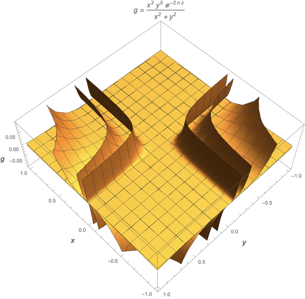
Plot3D with table for n dependence

It is based on the idea that the whole function set fits into a subregion of the unit cube. And it does bravely.

Plot[Table[g[x, 1, t, -1], {t, -2, 2, 1}], {x, -5, 5}, 
 PlotRange -> {All, {-25, 25}}]
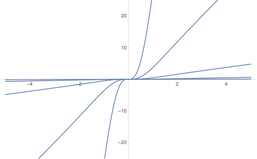
enter image description here

Table[Plot[Table[g[x, y, t, -1], {t, -2, 2, 1}], {x, -5, 5}, 
  PlotRange -> {All, {-25, 25}}], {y, -8, 8, 2}]
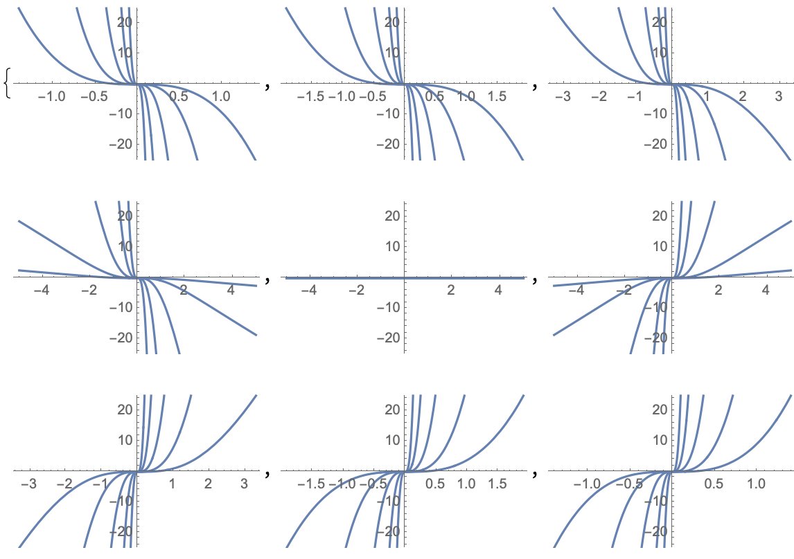
Plot table of inner tables in Plot

This question smoothing 3d contours as post processing has an interesting answer.

To return to normal plotting just use PlotPlots on the example given by @bob-hanlon and vary n. That confuses but does not help at all. Forget about the built-in grids on surface and use a personal selection following this ideas: plot a 2d vector path onto a surface. This question is about artefacts in 3d plots. There are more nice ideas.

I will come back later.

$\endgroup$

Not the answer you're looking for? Browse other questions tagged or ask your own question.