it's me again.
Strange stuff to report today. I suspect I've found a bug! Here is the nonlinear diffusion equation direct from the Mathematica documentation for FEM.
c = 1/Sqrt[(1 + Grad[u[x, y], {x, y}].Grad[u[x, y], {x, y}])];
Cu = {{{{c, 0}, {0, c}}}};
eqn = {Inactive[Div][
     Cu[[1, 1]].Inactive[Grad][u[x, y], {x, y}], {x, y}] == 0};
And a simple mesh to solve it with:
Needs["NDSolve`FEM`"];
mesh = ToElementMesh[FullRegion[2], {{-1, 1}, {-1, 1}}];
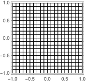
Show[mesh["Wireframe"], Frame -> True]
Note the exact solution (the diffusion tensor is constant for this case):
uA[x_, y_] = y;
Our boundary conditions will "target" this solution, using mixed Dirichlet and periodic boundary conditions (can do it with pure Dirichlet but that misses the point of this post):
bcs = {DirichletCondition[u[x, y] == uA[x, y], -1 < x < 1],
   PeriodicBoundaryCondition[u[x, y], x == 1, # - {2, 0} &]};
We provide the solver an initial guess (seed) that agrees on the boundary with the exact solution, but deviates inside. (This is not important, but we want the solver to work a bit for the solution.)
uSeed[x_, y_] = (1 - 0.3 (1 - x^2) (1 - y^2)) uA[x, y];
Now we solve this problem with NDSolveValue:
{ufA} = NDSolveValue[Join[eqn, bcs], {u}, Element[{x, y}, mesh],
  InitialSeeding -> {u[x, y] == uSeed[x, y]}];
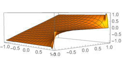
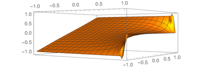
Plot3D[ufA[x, y], Element[{x, y}, mesh]]
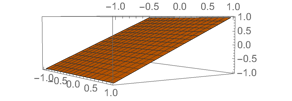
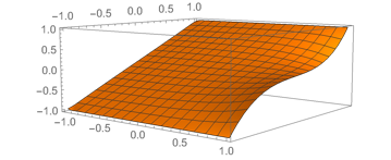
Oh dear! This doesn't look good! We wanted it to look this of course:
Plot3D[uA[x, y], Element[{x, y}, mesh]]
But, to the point now. It does not even satisfy the periodic boundary condition, on the target boundary x == 1! That is the problem, simply stated. What is going on here?
I will scratch a little deeper to gather some clues, using FEM programming. Just mostly copying code from the documentation here:
iSeeding = {uSeed[x, y]};
vd = NDSolve`VariableData[{"DependentVariables", "Space"} -> {{u}, {x, y}}];
sd = NDSolve`SolutionData[{"DependentVariables",
     "Space"} -> {iSeeding, ToNumericalRegion[mesh]}];
coefficients = {"DiffusionCoefficients" -> Cu};
initCoeffs = InitializePDECoefficients[vd, sd, coefficients];
initBCs = InitializeBoundaryConditions[vd, sd, bcs] ;
methodData =
  InitializePDEMethodData[vd, sd, Method -> {"FiniteElement"}];
linearizedPDECoeffs = LinearizePDECoefficients[initCoeffs, vd, sd];
{linLoadPDEC, linStiffnessPDEC, linDampingPDEC, linMassPDEC} =
  SplitPDECoefficients[linearizedPDECoeffs, vd, sd];
sdU = EvaluateInitialSeeding[methodData, vd, sd];
linear = DiscretizePDE[linearizedPDECoeffs, methodData,
  sdU]; {linearLoad, linearStiffness, linearDamping, linearMass} =
 linear["SystemMatrices"];
linearBCs = DiscretizeBoundaryConditions[initBCs, methodData, sdU];
seed = NDSolve`SolutionDataComponent[sdU, "DependentVariables"];
All standard stuff. Now we come to something interesting. We call DeployDirichletConditions on the seed data that we just created. The way we set up the boundary conditions, this should do nothing because the seed already satisfies the boundary conditions. It requires no modification. However it is indeed modified quite signifiantly:
{DeployDirichletConditions[seed, linearBCs],
 Norm@(seed - seedOLD)/Norm[seedOLD]}
{Null, 0.175549}
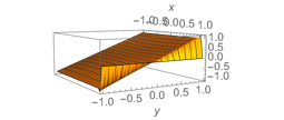
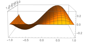
Now let's visualize the modified seed data:
uSeedf = ElementMeshInterpolation[mesh, seed];
Plot3D[uSeedf[x, y], {x, -1, 1}, {y, -1, 1}, AxesLabel -> Automatic]
This seems like an important clue. The seed has been modified so that the values at x==1 (the target of PeriodicBoundaryCondition) are now all zero (rather than periodic as they should be)! It seems something has gone wrong. To finish the solution, we need two functions femJacobian and femRHS, copied from the documentation, and I'll give their definitions at the end of this post for reference; you'll have to execute that them first. Then we run FindRoot to get the solution:
root = U /.
   FindRoot[femRHS[U], {U, seedOLD}, Jacobian -> femJacobian[U],
    Method -> {"AffineCovariantNewton"}];
NDSolve`SetSolutionDataComponent[sdU, "DependentVariables", root];
{uf} = ProcessPDESolutions[methodData, sdU];
Plot3D[uf[x, y], Element[{x, y}, mesh]]
The solution agrees with the one that came from NDSolveValue, as expected -- i.e. it's wrong. However, let's try FindRoot again, but this time circumvent the effect of DeployDirichletConditions by using the unmodified seed, seedOLD:
root = U /.
   FindRoot[femRHS[U], {U, seedOLD}, Jacobian -> femJacobian[U],
    Method -> {"AffineCovariantNewton"}];
NDSolve`SetSolutionDataComponent[sdU, "DependentVariables", root];
{uf} = ProcessPDESolutions[methodData, sdU];
Plot3D[uf[x, y], Element[{x, y}, mesh]]
This looks great! Time to celebrate? Sorry, not so fast. There are more problems. The solver seems to do OK if the initial seed agrees with the final solution on the target boundary (x==1). This is rather artificial. For many problems, we won't know what the solution will be on the boundary. For example, if we try the following seed function, things go very sour again:
uSeed[x_, y_] = (1 - 0.8 (1 - y^2)) uA[x, y];
This seed function is similar to the original, but it deviates from the exact solution when Abs[y] < 1, i.e. on the boundaries x==-1 and x==1. If we solve again (we have to go back to the definition of iSeed above), the standard way, with DeployDirichletConditions, we obtain the solution that violates periodicity (agres with the original output of NDSolveValue, uA). If we try our new "trick" and skip DeployDirichletConditions, things get interesting again:
Plot3D[uf[x, y], Element[{x, y}, mesh]]
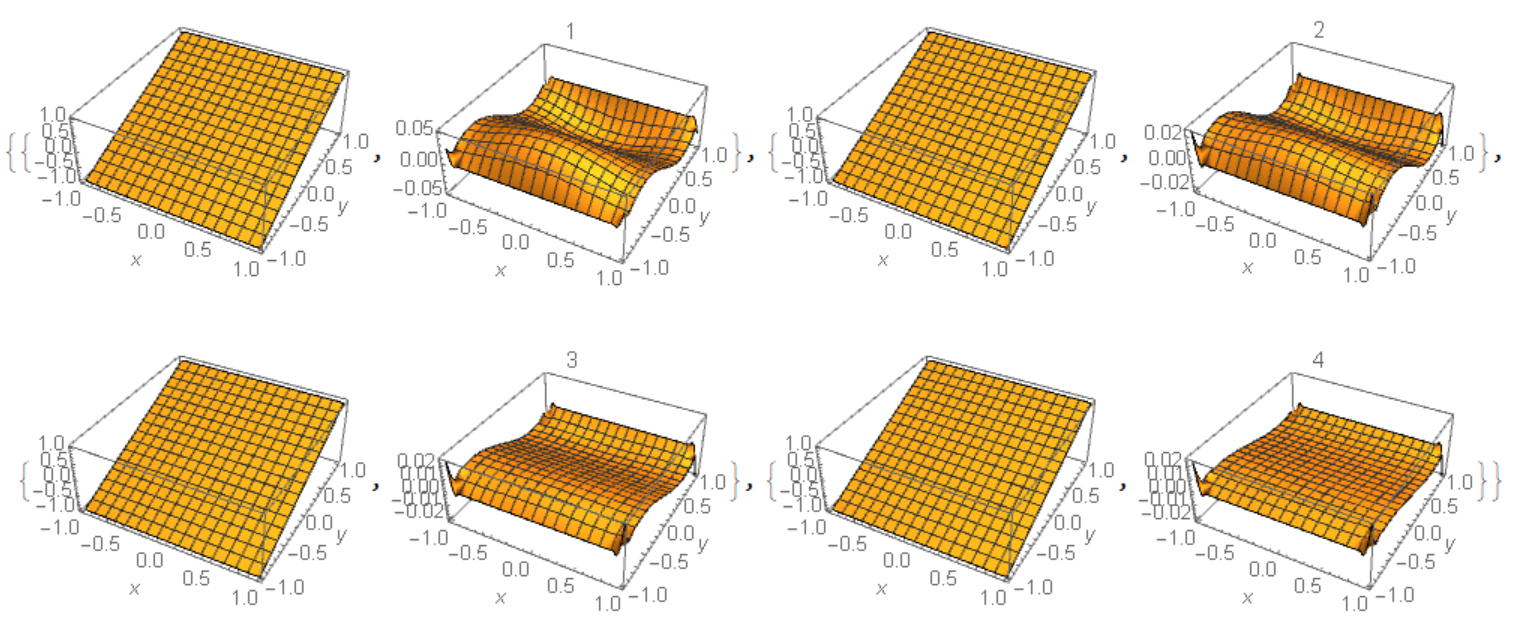
If we look at the solution near the x == 1 boundary it seems there is a remnant of the seed function. Indeed if we subtract the seed we find
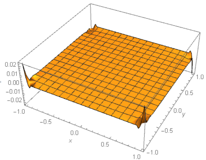
Plot3D[uf[x, y] - uSeed[x, y], Element[{x, y}, mesh], PlotRange -> All]
Instead of enforcing periodic BC, the solver is effectively forcing the solution to be equal to the seed function uSeed at the target boundary x == 1. This is very curious behavior! I really hope someone has an idea about this. @user21?
Below are the functions you need copied from the Mathematica documentation. Thanks for reading.
femRHS[u_?VectorQ] :=
  Block[{load, nonlinear, nonlinearLoad, nonlinearBCs},
   NDSolve`SetSolutionDataComponent[sdU, "DependentVariables", u];
   nonlinear =
    DiscretizePDE[linLoadPDEC, methodData, sdU, "Nonlinear"];
   nonlinearLoad = nonlinear["LoadVector"];
   nonlinear = Null;
   load = linearLoad + nonlinearLoad;
   nonlinearLoad = Null;
   (*subtract the linear Robin boundary value*)
   load -= linearBCs["StiffnessMatrix"].u;
   nonlinearBCs =
    DiscretizeBoundaryConditions[initBCs, methodData, sdU,
     "Nonlinear"];
   DeployPartialBoundaryConditions[{load, Null}, nonlinearBCs];
   DeployPartialBoundaryConditions[{load, Null}, linearBCs];
   load = -load;
   Normal[Flatten[load]]];

femJacobian[u_?VectorQ] :=
  Block[{stiffness, nonlinear, nonlinearStiffness, nonlinearBCs},
   NDSolve`SetSolutionDataComponent[sdU, "DependentVariables", u];
   nonlinear =
    DiscretizePDE[linStiffnessPDEC, methodData, sdU, "Nonlinear"];
   nonlinearStiffness = nonlinear["StiffnessMatrix"];
   nonlinear = Null;
   stiffness = linearStiffness + nonlinearStiffness;
   nonlinearStiffness = Null;
   nonlinearBCs =
    DiscretizeBoundaryConditions[initBCs, methodData, sdU,
     "Nonlinear"];
   DeployPartialBoundaryConditions[{Null, stiffness}, nonlinearBCs];
   DeployPartialBoundaryConditions[{Null, stiffness}, linearBCs];
   stiffness];

